
DEVELOPMENT OF A SINGLE PARTICLE MODEL … a kinetic study with a CFD model was ... Diffusion models...
231
Sede Amministrativa: Università degli Studi di Padova Dipartimento di Ingegneria Industriale SCUOLA DI DOTTORATO DI RICERCA IN INGEGNERIA INDUSTRIALE INDIRIZZO: INGEGNERIA CHIMICA, DEI MATERIALI E DELLA PRODUZIONE CICLO: XXVI STUDY OF NON CATALYTIC GAS-SOLID REACTIONS: DEVELOPMENT OF A SINGLE PARTICLE MODEL Direttore della Scuola : Ch.mo Prof. Paolo Colombo Coordinatore d’indirizzo: Ch.mo Prof. Enrico Savio Supervisore :Ch.mo Prof. Paolo Canu Dottorando : Tommaso Melchiori
Transcript of DEVELOPMENT OF A SINGLE PARTICLE MODEL … a kinetic study with a CFD model was ... Diffusion models...
Sede Amministrativa: Università degli Studi di Padova
Dipartimento di Ingegneria Industriale
SCUOLA DI DOTTORATO DI RICERCA IN INGEGNERIA INDUSTRIALE
INDIRIZZO: INGEGNERIA CHIMICA, DEI MATERIALI E DELLA PRODUZIONE
CICLO: XXVI
STUDY OF NON CATALYTIC GAS-SOLID REACTIONS:
DEVELOPMENT OF A SINGLE PARTICLE MODEL
Direttore della Scuola : Ch.mo Prof. Paolo Colombo
Coordinatore d’indirizzo: Ch.mo Prof. Enrico Savio
Supervisore :Ch.mo Prof. Paolo Canu
Dottorando : Tommaso Melchiori

1
Abstract
This thesis investigates single particle models to describe non catalytic gas-solid reactions. A comparative
study was made between the traditional shrinking core model and more detailed continuous models,
involving the solution of microscopic balances for the solid and gas phases inside a single porous particle.
Such a study proved that in some cases the use of the shrinking core model can lead to severe errors in the
prediction of conversion, and that kinetic parameters in SCM are affected by the particle size. Different
diffusion models were tested for the continuous model, and the inaccuracy of the Fick law compared to
multicomponent Stefan-Maxwell was evaluated, depending on the concentration of the reaction gas in the
mixture. The thesis also proved that natural convection inside the particle can be neglected by changing the
balance from mass to molar basis or vice versa, depending on the type of reaction considered. An equation
for the local particle porosity was also included, to account for the local changes of gas diffusivity as effect
of the reaction. The effect of the pore size distribution was studied, by writing the particle model as a
population balance, including different diffusive resistances for different pore sizes, for the cases when
Knudsen or solid state diffusion can be important. Sintering phenomena were included, by extending the
grain model with an empiric equation. Simulations with simultaneous gas solid reactions were performed,
also considering non uniform initial distributions of the solid phases inside the particle: sensitivity studies
proved that the position of the solid reagents in the particle may have a great influence on the model
results, even when intra particle diffusion is fast compared to the chemical reactions. Gas-solid models
were also used to simulate real processes. In particular, thanks to collaboration with an industrial research
project, a kinetic study with a CFD model was developed, applying a shrinking core model to simulate real
reactors for the direct reduction of iron ores with syn gas at high temperature and pressure. Finally, thanks
to the collaboration with the Technical University of Eindhoven, a continuous model was used to simulate
reactions of reduction of iron-titanium oxides in chemical looping combustion processes, comparing the
results with experimental data.

2
3
Riassunto
Questa tesi investiga modelli di singola particella per descrivere reazioni gas-solido non catalitiche. E’ stato
fatto uno studio comparativo fra il tradizionale shrinking core model e modelli continui più dettagliati che
comprendono la risoluzione dei bilanci microscopici per le fasi gas e solida dentro una singola particella
porosa. Tale studio ha provato che in alcuni casi lo shrinking core model può condurre ad errori importanti
nella predizione della conversione, e che i parametri cinetici nel SCM dipendono dalla dimensione della
particella. Sono stati testati diversi modelli di diffusione all’interno del modello continuo, e la non
accuratezza della legge di Fick rispetto alla Stefan-Maxwell multicomponente è stata valutata, a seconda
della concentrazione del gas reagente nella miscela. La tesi prova anche che la convezione naturale
all’interno della particella può essere trascurata cambiando i bilanci da massivi a molari o vice versa, a
seconda del tipo di reazione considerata. Un’equazione che descrive la porosità locale della particella è
stata inclusa al modello, per tener conto dei cambiamenti della diffusività effettiva del gas per effetto della
reazione. L’effetto della distribuzione della dimensione dei pori è stato investigato, riscrivendo il modello di
particella come bilancio di popolazione, includendo diverse resistenze diffusive per diverse dimensioni dei
pori, per i casi in cui La diffusione di Knudsen o la diffusione in stato solido possono essere importanti.
Fenomeni di sinterizzazione sono stati inclusi, estendendo il tradizionale grain model con un’equazione
empirica. Sono state fatte simulazioni di reazioni gas solido con più reazioni, considerando anche
distribuzioni disomogenee delle fasi solide all’interno della particella: studi di sensitività hanno dimostrato
che la posizione dei reagenti solidi nella particella possono avere un effetto importante sui risultati del
modello, anche nel caso in cui la diffusione all’interno della particella è veloce rispetto alle reazioni
chimiche. Modelli di reazione gas-solido sono stati usati anche per simulare processi reali. In particolare,
grazie alla collaborazione con un progetto di ricerca industriale, uno studio cinetico con modelli CFD è stato
sviluppato, applicando lo shrinking core model per simulare reattori reali per la riduzione diretta di ossidi di
ferro con gas di sintesi ad alte temperature e pressioni. Infine, grazie alla collaborazione con l’Università
Tecnica di Eindhoven, un modello continuo è stato usato per simulare reazioni di riduzione di ossidi di
ferro-titanio in processi di chemical looping combustion, confrontando i risultati con i dati sperimentali.

4
5
Contents
Abstract ...................................................................................................................................................... 1
Riassunto .................................................................................................................................................... 3
Chapter 1. Introduction ....................................................................................................................... 9
Chapter 2. The shrinking core model ................................................................................................ 13
2.1 Shrinking Core Model for cylindrical particles ......................................................................... 19
2.2 Shrinking Core Model for time changing particle size ............................................................. 21
2.3 Shrinking Core Model for a reversible reaction....................................................................... 23
2.4 Multiple interfaces Shrinking Core .......................................................................................... 25
2.5 Limitations of the Shrinking Core Model ................................................................................. 30
Notation ............................................................................................................................................... 31
Chapter 3. Application of SCM: Simulation of full scale reactors for Direct Reduction of Iron ........ 33
3.1 Model overview ....................................................................................................................... 33
3.2 Mathematical model used in CFD ........................................................................................... 34
3.3 Model results ........................................................................................................................... 35
3.4 Conclusions .............................................................................................................................. 40
Chapter 4. Continuous Models .......................................................................................................... 43
4.1 Material balances .................................................................................................................... 43
4.2 Energy balance......................................................................................................................... 46
4.3 Model for spherical particles ................................................................................................... 49
4.4 Boundary and initial conditions ............................................................................................... 51
4.5 Reaction models ...................................................................................................................... 52
4.5.1 Effect of the gas concentration ........................................................................................... 53
4.5.2 Effect of solid conversion .................................................................................................... 55
4.5.3 Effect of chemical equilibrium ............................................................................................. 57
4.6 Continuous model in terms of mass ........................................................................................ 58
Notation ............................................................................................................................................... 59
Chapter 5. Diffusion models .............................................................................................................. 61
5.1 Gas diffusion and velocity ........................................................................................................ 61
5.2 Binary and multicomponent diffusion: Fick and Stefan-Maxwell ........................................... 63
5.3 Other forms of the Stefan-Maxwell equations ........................................................................ 66
5.3.1 From multicomponent to binary form ................................................................................ 70
5.3.2 Alternative (direct) way to derive SM-equation in term of massive fluxes......................... 71
6
5.4 Contribution of Knudsen diffusion .......................................................................................... 71
5.5 Generalized Stefan-Maxwell for multiple driving forces and non ideal solutions .................. 72
5.6 Simplified diffusion models: Mixture averaged model ........................................................... 73
5.6.1 Derivation of mass fluxes .................................................................................................... 74
5.7 Effective diffusion coefficients ................................................................................................ 75
Notation ............................................................................................................................................... 75
Chapter 6. Role of diffusion and convection in particle models ....................................................... 77
6.1 Mathematical proof of model simplifications ......................................................................... 77
6.2 Sensitivity analysis on diffusion models .................................................................................. 79
6.2.1 Effect of the fraction of inert ............................................................................................... 81
6.2.2 Effect of the controlling regime ........................................................................................... 84
6.2.3 Effect of non homogeneous diffusion matrix ...................................................................... 85
6.3 Role of convection ................................................................................................................... 88
6.3.1 Gas equimolar reaction: reduction of wustite .................................................................... 89
6.3.2 Gas non equimolar reaction: oxidation of zinc sulphide ..................................................... 93
6.3.3 Effect of convection in kinetic regime ................................................................................. 98
Notation ............................................................................................................................................... 99
Chapter 7. Particle models for Chemical Looping Combustion ....................................................... 101
7.1 Chemical Looping Combustion .............................................................................................. 101
7.2 Experimental estimation of carriers reactivity: TGA analysis ................................................ 103
7.3 Application of the Shrinking Core Model .............................................................................. 105
7.4 Modified grain model ............................................................................................................ 108
7.5 Effect of pore size distribution .............................................................................................. 112
7.5.1 Application to CLC experimental data: reduction of CuO ................................................. 115
7.5.2 Model results ..................................................................................................................... 118
7.6 Effect of gas diffusion in dense solid ..................................................................................... 121
7.7 Effect of solid phases segregation ......................................................................................... 124
7.7.1 Model development .......................................................................................................... 125
7.7.2 Model predictions and sensitivity to non uniform initial conditions ................................ 127
7.7.3 Simulation of the experimental data ................................................................................. 138
Notation ............................................................................................................................................. 143
Chapter 8. Comparison between the Shrinking Core Model and the Continuous Model .................. 145
8.1 Description of the compared models .................................................................................... 146
8.1.1 Continuous model ............................................................................................................. 146
8.1.2 Shrinking core model ......................................................................................................... 149
7
8.2 Comparison of the two models ............................................................................................. 151
8.2.1 Diffusive regime ................................................................................................................. 152
8.2.2 Kinetic regime .................................................................................................................... 153
8.2.3 Intermediate regime .......................................................................................................... 161
8.3 Particle size issues ................................................................................................................. 163
8.4 Conclusion ............................................................................................................................. 166
Notation ............................................................................................................................................. 167
Chapter 9. Coupling of particle models with reactor models ......................................................... 169
9.1 Solution for a simplified continuous model .......................................................................... 171
9.2 Coupling with 1D moving bed reactor model ........................................................................ 175
Notation ............................................................................................................................................. 178
Chapter 10. Conclusions .................................................................................................................... 181
Appendix A: Numerical discretization of the continuous model by Finite Differences ......................... 185
Calculation of the matrices ................................................................................................................ 187
Diffusive term ................................................................................................................................. 188
Generalization of the diffusion matrix D ........................................................................................ 189
Convection term ............................................................................................................................. 190
Jacobian matrix and source term ................................................................................................... 190
Appendix B: Basics of Weighted Residual Methods ............................................................................... 193
WRM for unsteady state problems .................................................................................................... 195
Boundary and initial conditions ......................................................................................................... 197
Appendix C: Matlab codes ...................................................................................................................... 199
Appendix D: Fortran codes ..................................................................................................................... 217
References .............................................................................................................................................. 225

8
9
Chapter 1. Introduction
The occurrence of reacting porous solids in many industrial applications is impressive. They span well
beyond the traditional chemical and metallurgical areas, to the energy production (coal, biomass),
agrochemicals, food and pharmaceuticals, aerospace propulsion and others. Processes involving reactions
with gases are more common than liquids; in this thesis, the study was focused on gas-solids applications.
The reaction systems concerned are of considerable industrial importance and are readily found in
chemical and metallurgical industries. Examples are the reduction of iron oxide or the oxidation of iron by
steam, the roasting and smelting of ores, the combustion of solid fuels and solid propellant, the gasification
of coal, the regeneration of catalysts, just to mention a few.
These systems involving heterogeneous reactions can occur in various types of reactors. In general, they
are usually extremely complex, and the experimental campaigns carried out to estimate the intrinsic
kinetics can easily fail to reveal the true mechanism because of the great number of variables involved. The
successful determination of such variables, and the consequent design of a reactor depend greatly on the
knowledge of reliable rate data. The rates of heterogeneous reactions often depend on the conditions
under which the experiment is performed. Physical effects such as diffusion and heat transfer can result in
an erroneous rate expression if they are not properly accounted for. The order of reaction, the activation
energy, and the selectivity determined may be so misleading that, if used in scale-up, the result may lead to
severe errors. It is therefore important to make a careful study of the interaction and to account for both
physical effects and purely chemical processes in a correct way. Even for an isothermal reaction system, the
overall reaction rates are influenced by the rate of chemical reactions occurring in or at the surface of a
solid, by the mass transfer rates of fluids through the solid as well as across the fluid-film surrounding the
solid. Besides, other factors can play a role, which are more strictly related to the properties of the porous
matrix, such local pore size and surface characteristics, but also solid reactivity of crystallite orientation,
crystallite size, etc. The description is further complicated by the fact that all of these characteristics can
change in time. This change can be caused by external stresses, by high temperature sintering, or, more
simply, by the chemical reaction itself. The transformation of the solid phase into a new one, with different
molar volume, modifies the morphology of the solid on the scale of the pores, and sometimes the whole
pellet.
For these reasons, a rigorous treatment seems very difficult to obtain, even for the solid of the simplest
geometry. Besides, a great number of difficult problems exist in practical systems, such as the changing size
and shape of the solid during the reaction and formation of a product around the solid reactant. Finally, the
complex velocity profile of the surrounding fluid makes the problems of mass and energy transfers to the
solid reactant more difficult to analyze.
The porous solid particles treated industrially are generally porous pellets. For a general reaction, involving
both a solid and a gas phase in both reagents and products, the physical steps concerning the gas in the
process are the following:
(i) Transfer within the external gas to the surface of the pellet.
(ii) Diffusion through the intergranular pores.
Chapter 1
10
(iii) Adsorption into the solid reacting phase.
(iv) Reaction at the gas/solid interface.
(v) Desorption of the produced gas.
(vi) Diffusion of the product gas to the external particle surface.
(vii) Transfer of the produced gas from the particle surface to the bulk gas.
Each of these steps has its own kinetics and can limit, also in part, the overall rate of conversion. The
process can be successfully described either as a chemical regime, when a surface process controls the
overall kinetics, or as a diffusional regime when the rate is determined by diffusion, or as a mixed regime.
If the reaction is exo- or endothermic, or if the external temperature varies, the associated heat evolution
or consumption phenomena, and heat transfer both within the pellet and with the exterior can have an
influence on all of the mentioned steps.
In the literature, these issues have partly been discussed, and in many cases, some simplifications are
assumed, in order to formulate models that are applicable to the description of full scale reactors, as much
as possible. A very comprehensive, classical treatment of the subject is the seminal book of Szekely[1]. In
spite of the impact, the quantitative treatment of reactive solids remains predominantly based on
oversimplification of the actual physics, that can be extremely complicated by the already mentioned
issues.
Looking at the different models that have been developed to describe non catalytic gas-solid reactions, two
main approaches can be identified. The most rigorous one requires solving the microscopic conservation
equations for the gas and the solid species within the single particle. According to this, the porous phase is
treated as pseudo-homogeneous continuous phase, with a local porosity, and a local concentration of
accessible surface per unit volume [2]. Important examples of these kind of continuous models are the
volumetric model[3], the grain model[1], the sintering model[4] and the random pore model[5, 6]. The
main difference between these is the dependency of the expression of the reaction rate on the solid
reactant concentration, as Gomez-Barea and Ollero tried to classify[7]. Different degree of detail can also
derive from the choice of the terms to include into the microscopic balances. Patisson et al.[8] pointed out
the importance to include the gas convection generated by non equimolar reactions. Valipour et al.[9]
remarked the difference that can arise while assuming pseudo steady state for the gas species with respect
to the solid phase, particularly when simulating particles in non isothermal conditions. Different diffusion
models can be considered, from the more rigorous Stefan Maxwell model[8], to a binary Fick[10], with
diffusivity possibly dependent on the gas composition[9]. Most of the authors agree that Knudsen diffusion
must also be taken into account together with molecular diffusion, with an effective coefficient depending
on the porosity of the particle.
A more simplified approach assumes non-porous particles[11], or non-porous shrinking core model
(SCM)[12]. The latter is widely used. According to it, the reaction is supposed to take place only on a
surface separating the unreacted core by the product layer in the particle, and moving to the center as the
reaction goes on. This physical description is not always correct, and in general it is not predictable whether
or not a gas-solid reaction occurs by forming a core-shell structure, because that depends on the reaction
conditions (structure and size of the particle, temperature, pressure, composition of the fed gas, etc). Even
with this limitation, the SCM is still widely used [13-18], as it provides a simple analytical solution for most
Introduction
11
cases, and it can still account for the presence of mass transfer resistances inside and outside the reacting
solid, even if in a simplified way.
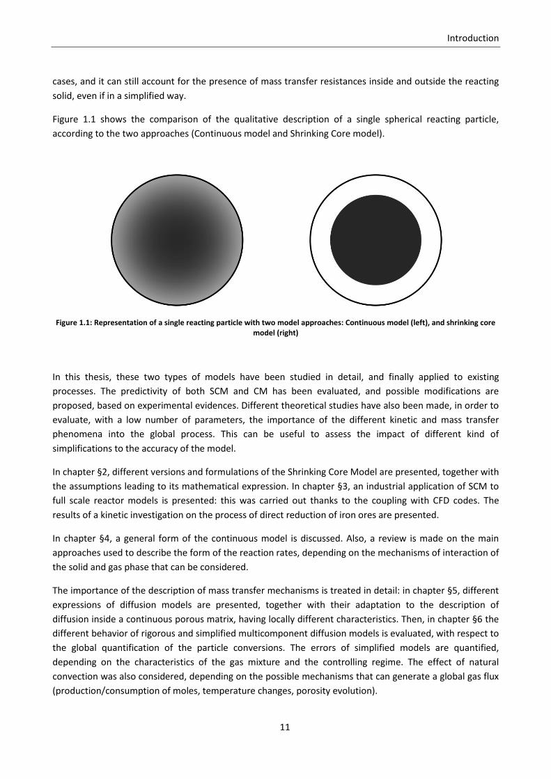
Figure 1.1 shows the comparison of the qualitative description of a single spherical reacting particle,
according to the two approaches (Continuous model and Shrinking Core model).
Figure 1.1: Representation of a single reacting particle with two model approaches: Continuous model (left), and shrinking core model (right)
In this thesis, these two types of models have been studied in detail, and finally applied to existing
processes. The predictivity of both SCM and CM has been evaluated, and possible modifications are
proposed, based on experimental evidences. Different theoretical studies have also been made, in order to
evaluate, with a low number of parameters, the importance of the different kinetic and mass transfer
phenomena into the global process. This can be useful to assess the impact of different kind of
simplifications to the accuracy of the model.
In chapter §2, different versions and formulations of the Shrinking Core Model are presented, together with
the assumptions leading to its mathematical expression. In chapter §3, an industrial application of SCM to
full scale reactor models is presented: this was carried out thanks to the coupling with CFD codes. The
results of a kinetic investigation on the process of direct reduction of iron ores are presented.
In chapter §4, a general form of the continuous model is discussed. Also, a review is made on the main
approaches used to describe the form of the reaction rates, depending on the mechanisms of interaction of
the solid and gas phase that can be considered.
The importance of the description of mass transfer mechanisms is treated in detail: in chapter §5, different
expressions of diffusion models are presented, together with their adaptation to the description of
diffusion inside a continuous porous matrix, having locally different characteristics. Then, in chapter §6 the
different behavior of rigorous and simplified multicomponent diffusion models is evaluated, with respect to
the global quantification of the particle conversions. The errors of simplified models are quantified,
depending on the characteristics of the gas mixture and the controlling regime. The effect of natural
convection was also considered, depending on the possible mechanisms that can generate a global gas flux
(production/consumption of moles, temperature changes, porosity evolution).
Chapter 1
12
In chapter §7, a continuous model approach is used to try to explain the experimental data of reduction of
solids in chemical looping combustion processes. Different interpretations are formulated, based on the
available evidences, and related to the detailed description of the solid matrix. In particular, they involve
the inclusion of sintering, non uniform pore size distribution, gas diffusion in dense solid, effect of solid
phase segregation, gas adsorption mechanisms.
In chapter §8, a comparative study between the Shrinking Core Model and the Continuous Model is shown.
A mathematical function was found to relate the parameters used in the two approaches, so that the
simplified SCM can better match the results of the continuous model. Also, the errors made with the SCM
are evaluated, as a function of the process conditions.
Finally, in chapter §9, a numerical technique is elaborated to couple the mathematical description of the
single particle to reactor models, based on polynomial collocation methods. Also, a simple PDE coupling is
shown for the case of a one dimensional moving bed reactor.
13
Chapter 2. The shrinking core model
Let’s consider a solid particle where a single gas-solid reaction occurs, in the form:
a A(s) + b B(g) c C(s) + d D(g)
One simple way of describing the reaction of a solid particle with a gas is by using the shrinking core model
[12, 19, 20]. The main assumption of this model is that the reaction develops topochemically, only on a
single surface which separates two zones within the solid. An unreacted core, made of pure solid reagent,
which has not been reached by the reacting gas yet, and a reacted outer layer, made of pure solid product,
which is porous, and where the gas diffuses but doesn’t react, because the solid matrix is completely inert.
The core shell interface moves inward, as long as the core is consumed, and the shell becomes thicker. This
concept can be applied to different particle geometries. For spherical pellets, the core shell interface is a
spherical surface concentric to the external one.
One advantage of assuming a core-shell type reaction is that the global conversion of the single particle is
simply related to the position of the core-shell interface. The conversion is in fact defined as:
2.1
Where n is the number of moles of the reagent solid into the particle. If the reagent is present only in the
core, then the amount of reagent in the particle is linearly related to the volume of the core, via the
reagent density:
2.2
So, combining equations 2.1 and 2.2 the particle conversion is:
2.3
As a function of the pellet radius:
2.4
The inverse function of equation 2.4 that gives the interface position as a function of the global conversion:
2.5
Chapter 2
14
If the layer is completely occupied by the solid product, the reagent gas only diffuses through it, without
reacting. So the microscopic balance for the gas species B and D will be:
2.6
2.7
In this model, the reaction appears in the boundary conditions, which are:
2.8
2.9
2.10
2.11
Where R is the superficial reaction rate occurring at the interface ri. At the core shell interface, the molar
flux of the single species is equal to the its superficial production rate (equations 2.8 – 2.9). At the particle
surface, the molar fluxes of the gas species are equal to those calculated considering the external mass
transfer resistance (equations 2.10 – 2.11). This is done by considering the mass transfer coefficients for
each component.
The total molar flux N is given by the total concentration balance, which is the sum of equations 2.6 and 2.7
if the gas mixture is made only by species B and D.
2.12
The boundary conditions for this equation are also found by summing equations 2.8-2.9 and 2.10-2.11,
respectively:
2.13
2.14
The total concentration of the solid species can be obtained by adding the global solid material balances to
the system of equations 2.6-2.7. The equations for species A and C are:
2.15
2.16
The shrinking core model
15
It’s important to note that in this notation CA and CC are the concentration of A and C considering the whole
particle volume, whereas cB and cD are the local concentration of gas B and D, and are variable with r. The
local concentration profiles of the solid (cA(r) and cC(r)) are already solved once the interface position ri is
known. In fact they will be:
2.17
2.18
Where is the initial concentration of A (assuming that the particle composition is initially uniform), and
is the Heaviside function, which is equal to one if and is equal to zero otherwise. In other
words, the solutions for the solids are step functions. Equation 2.12 can also be written in terms of particle
conversion X, as follows:
2.19
So, equation 2.19 can be solved to calculate the interface position ri at the current time, by also using
equation 2.5. This is necessary because ri is involved in the boundary conditions for the gas equations (2.8,
2.9, 2.13).
The system of equations for the gas and solid can be easily solved, by considering a number of possible
simplifications. First of all, the total concentration balance 2.12 can be neglected, in the following
conditions: if the layer solid structure is uniform, then the layer porosity is radially homogeneous; if the
temperature and pressure of the gas inside the particle are also constant, then the total gas concentration
is constant; so the time derivative into equation 2.8 is then equal to zero, which means that the total molar
flux N is:
2.20
In particular, if d = b (gas equimolar reaction), the total molar flux is constantly zero. The diffusive fluxes of
the gases can be expressed by the Fick’s law, if the mixture is binary. If the total gas concentration is also
constant (uniform temperature and pressure), then the fluxes are:
2.21
2.22
The diffusivity DBD is an effective coefficient, that depends on the local porosity and tortuosity of the
medium. If the solid structure of the layer is uniform, and gas pressure and temperature are also constant
with the radial coordinate, DBD is constant, and can be calculated as:
Chapter 2
16
2.23
Where is the molecular binary diffusion coefficient of species B in D (that of the gas mixture out of the
solid matrix). A final hypothesis can be made in order to further simplify the material balances in equations
2.6-2.7. The time variation of the gas concentration profiles is usually very fast if compared to the time
variation of the interface position (and consequently of the solid conversion). In this situation, the time
derivatives in equations 2.6-2.7 are not very important, and the gas balances can be solved in steady state
at a given core-shell interface position, ri. This doesn’t mean that the gas concentration profiles are not
time-dependent, because their balances are still coupled with the solid equations, where the time
derivatives are still present.
The system of equations can be solved, once the expression of the kinetic rate is defined. For a single,
irreversible, first order reaction, it is:
2.24
Where k’ is the superficial kinetic constant. With all the mentioned assumptions, the system of equations
for the gas and solid reagents to solve is:
2.25
2.26
With the boundary and initial conditions:
2.27
2.28
2.29
Equation 2.25 can be easily integrated, giving:
2.30
In this equation, A and B are integration constants, that can be calculated by imposing the boundary
conditions 2.27-2.28. Applying equation 2.30 to equations 2.27-2.28 we obtain:
2.31
2.32
The shrinking core model
17
A linear system in A and B is obtained:
2.33
Whose solution is:
2.34
2.35
So, the complete solution can be found by using equations 2.34-2.35 into equation 2.30. The result is the
following:
2.36
The explicit solution for the gas concentration profile can be found only for a first order kinetic expression.
Thanks to equation 2.36, the concentration of the gas reagent at the interface position can be calculated
analytically, as a function to the gas bulk concentration outside the particle. For r = ri, we obtain:
2.37
This concentration can be applied to equation 2.26 to calculate the evolution of the global particle
conversion in time. The resulting differential equation in time becomes:
2.38
Finally, using equation 2.5 into equation 2.38 the variable ri can be replaced by its function of the
conversion X, so we get to an equation with only one dependent variable:
2.39
Chapter 2
18
Equation 2.39 is the shrinking core model equation for a spherical particle, considering a single irreversible
reaction. It is a very useful model, because it can give the change of the particle conversion as a function of
the bulk gas reactant concentration alone. So, no information about the inner gas concentration profiles is
necessary to solve it. This is quite important because it can be easily applied to simulate systems where a
high number of reacting particles is involved. The shrinking core model can be coupled with a gas
concentration balance solved in the inter particle channels, that can provide the value of as a
function of time. If is constant (this is the case when a high gas flowrate is fed around the particle at
a constant composition), equation 2.39 has an analytical solution, which is:
2.40
The parameters , , are the characteristic times related to the kinetic, diffusive and external mass
transfer resistances, respectively, which are defined by equations 2.41-2.43.
2.41
2.42
2.43
The values of the characteristic times are related to the importance of their respective resistances in the
process. For instance a high value of means that diffusion is not negligible, and in fact it can be related
to a low value of the diffusion coefficient. To understand which is the controlling regime it is useful to
calculate the ratios between the characteristic times. In particular two non dimensional numbers can be
defined: Damkohler, which is the ratio between the diffusive and kinetic times, and Biot, which is the ratio
between the diffusive and mass transfer characteristic times:
2.44
2.45
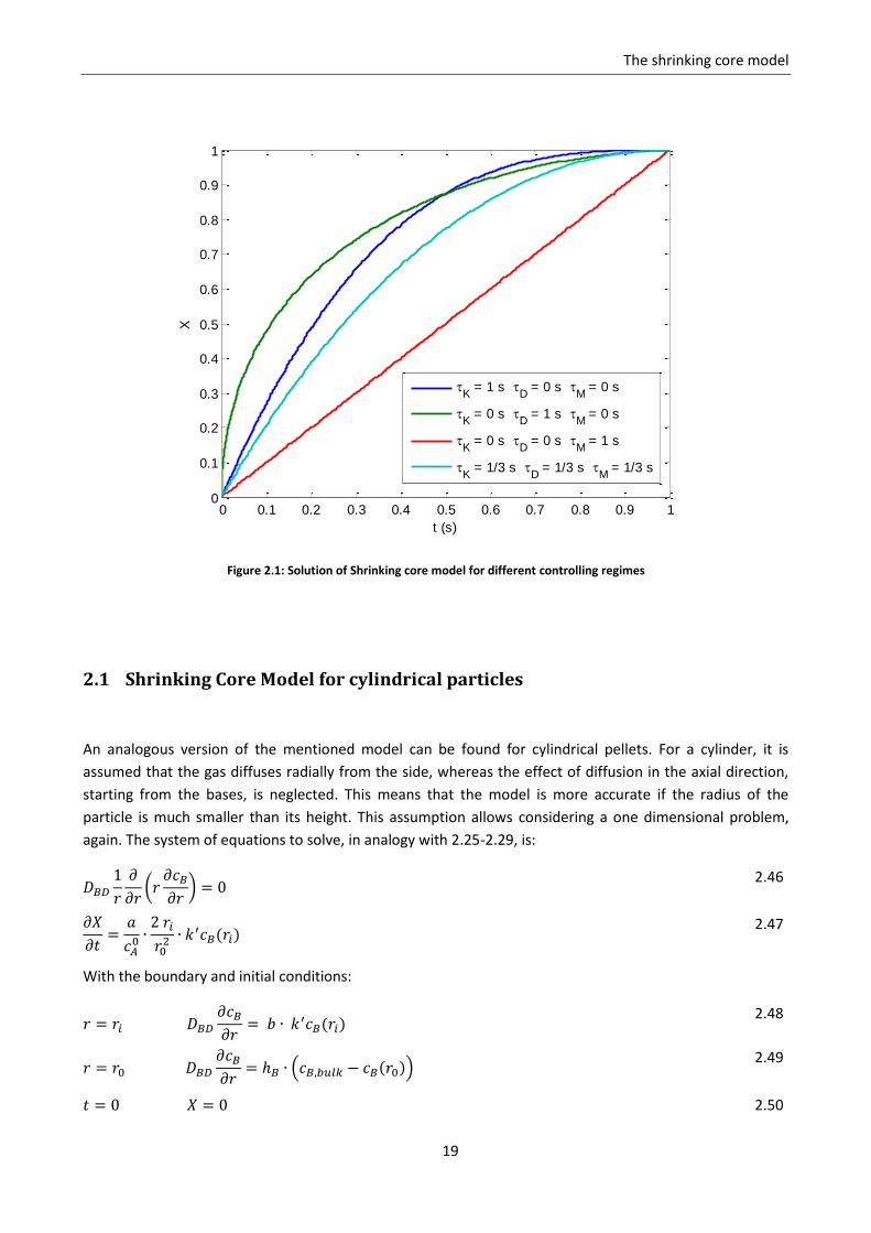
Figure 2.1 shows the results of the shrinking core model obtained by equation 2.40 for three different
controlling regimes.
The shrinking core model
19
Figure 2.1: Solution of Shrinking core model for different controlling regimes
2.1 Shrinking Core Model for cylindrical particles
An analogous version of the mentioned model can be found for cylindrical pellets. For a cylinder, it is
assumed that the gas diffuses radially from the side, whereas the effect of diffusion in the axial direction,
starting from the bases, is neglected. This means that the model is more accurate if the radius of the
particle is much smaller than its height. This assumption allows considering a one dimensional problem,
again. The system of equations to solve, in analogy with 2.25-2.29, is:
2.46
2.47
With the boundary and initial conditions:
2.48
2.49
2.50
0 0.1 0.2 0.3 0.4 0.5 0.6 0.7 0.8 0.9 10
0.1
0.2
0.3
0.4
0.5
0.6
0.7
0.8
0.9
1
t (s)
X
K = 1 s
D = 0 s
M = 0 s
K = 0 s
D = 1 s
M = 0 s
K = 0 s
D = 0 s
M = 1 s
K = 1/3 s
D = 1/3 s
M = 1/3 s
Chapter 2
20
The general solution of equation 2.46 is:
2.51
Using the boundary conditions, A and B are found by solving the system:
2.52
Whose solution is:
2.53
2.54
The gas reagent concentration profile inside the solid product layer, at a given core-shell position interface,
results as follows:
2.55
If r = ri, we obtain the analytical expression of the gas concentration at the reaction interface, as a function
of the bulk concentration, decreased for effect of the three resistances:
2.56
So the differential equation to solve to get the global particle conversion is:
2.57
Or, as a function of the conversion alone:
2.58
The shrinking core model
21
Again, equation 2.58 can be easily integrated if is constant in time: the solution of the shrinking core
model for a cylindrical geometry, for one single irreversible reaction is:
2.59
Where the characteristic times are:
2.60
2.61
2.62
2.2 Shrinking Core Model for time changing particle size
The analysis made so far assumed that the particle radius, r0, remains constant as long as the reaction
proceeds. This is not always true. The loss or gain of mass of the solid during the reaction, the layer porosity
and the restructuring of the product to a crystal structure with different density can lead to a change of the
particle size. The total volume of the particle can be calculated at any time by considering a total mass
balance. The volume of the core, VA, can be obtained as a function of the conversion by using equation 2.5:
2.63
Where r0(0) is the particle radius at t = 0. Consequently, the number of moles of the solid reactant A in the
particle is:
2.64
According to stoichiometry, the number of moles of the product C must be the number of reacted moles of
A, scaled by the ratio between the coefficients c and a. SO it will be:
2.65
So the volume occupied by the product C, which is equal to the volume of the layer according to the
shrinking core model, can be calculated as follows:
Chapter 2
22
2.66
The total particle volume can be calculated by the sum of equations 2.63 and 2.66:
2.67
So the particle radius, as a function of the conversion is:
2.68
Where:
2.69
Depending on the value of ψ, three situations are possible:
- If ψ > 0: the particle increases in volume with conversion.
- If ψ = 0: the particle size remains unchanged.
- If ψ < 0: the particle volume decreases with conversion.
It’s important to point out that ρC is the apparent density of the product phase, so it takes into account the
porosity of the layer: this means that ρC will be, in general, lower than the intrinsic density of the product C.
The evolution of the particle porosity can be independent from the intrinsic properties of the solid phases
involved in the reaction, and this means that the quantification of ψ can be non trivial.
The particle shrinking and swelling can have an influence on the process, because the diffusion resistance is
related to the thickness of the layer. For a spherical particle, equation 2.39 is still valid, but r0 is not a
constant in the integration, but a function of the conversion, as stated by equation 2.68. So the model
becomes:
2.70
Analogously, for a cylindrical pellet, the particle radius will be:
2.71
So the shrinking core model becomes:
The shrinking core model
23
2.72
2.3 Shrinking Core Model for a reversible reaction
The models previously presented consider that the reaction at the core shell interface is irreversible, so it
only depends on the concentration of the gas reagent. Now let’s consider the case where the equilibrium
reaction is involved:
a A(s) + b B(g) ↔ c C(s) + d D(g)
If equilibrium is involved, the concentration balance for the product gas D must be coupled with the system
of equations. For a spherical particle it is:
2.73
2.74
2.75
With the boundary and initial conditions:
2.76
2.77
2.78
Like the solution for the irreversible reaction case, the gas reagent and product concentration profiles are
in the form:
2.79
2.80
Four integration parameters need to be found by applying the four boundary conditions in 2.76-2.77:
Chapter 2
24
2.81
2.82
2.83
2.84
A linear system in A1, A2, B1 and B2 is obtained:
2.85
Solving the system, the concentrations of B and D at the reaction interface can be found. Equation 2.75
becomes:
2.86
And, expressing the interface position in terms of conversion:
2.87
Comparing this expression with the model for irreversible reaction, two more resistances appear in
equation 2.87: they are related to the diffusion of the product gas in the layer and the mass transfer of the
product from the particle surface to the bulk. It is trivial to prove that if K tends to infinite (the equilibrium
is completely shifted to the products) equation 2.87 becomes identical to equation 2.39. Equation 2.87 can
be further generalized, in the case that the gas B and D are not in a binary mixture, but are diluted in an
inert species, I. The Fick law is still applicable on the problem, if the fractions of B and D are small if
The shrinking core model
25
compared to the fraction of inert. In this case, the diffusion coefficient DBI and DDI of the reagent and
product into the inert gas can be sometimes very different from each other. An equation for the global
particle conversion can still be found, analogously to what already reported. The final solution is:
2.88
This model can also be extended to describe particles with changing size, by expressing r0 through equation
2.68.
2.4 Multiple interfaces Shrinking Core
The shrinking core model can be extended to consider for multiple reactions [21] [19], in the case that the
solid product of the first reaction can further react with the same gas. The model predicts the formations of
multiple layers, surrounding a core made of the first solid reagent. In this section it is reported the case for
two reactions, assuming that the same gas reagent and product are involved in both reactions:
a A(s) + b1 B(g) ↔ c1 C(s) + d1 D(g)
c2 C(s) + b2 B(g) ↔ e E(s) + d2 D(g)
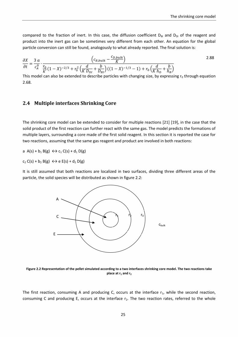
It is still assumed that both reactions are localized in two surfaces, dividing three different areas of the
particle, the solid species will be distributed as shown in figure 2.2:
Figure 2.2 Representation of the pellet simulated according to a two interfaces shrinking core model. The two reactions take place at r1 and r2
The first reaction, consuming A and producing C, occurs at the interface r1, while the second reaction,
consuming C and producing E, occurs at the interface r2. The two reaction rates, referred to the whole
r0
r2
r1
cbulk
A
C
E
Chapter 2
26
particle volume, can be expressed through equations 2.89 -2.90. Once again they consider first order
dependence on the gas concentrations:
2.89
2.90
The goal is once again to express the concentrations of B and D at the two interfaces as a function of the
bulk concentrations outside the particle. Again, the material balances for the gas species B and D only
consider diffusion through the solid matrices, but it’s possible that the effective diffusivities of the gases in
the layers with species C and species E are different from each other. This is true, for instance, if the layers
have different porosities. In this case the model for the gas is:
2.91
2.92
In this case, and
are the effective diffusivities of B inside the layer occupied by the solid C and E,
respectively. An analogous pair of coefficients, and
are defined for the gas product D. For the solid
species, the total concentrations of A and C in the particle can be expressed through the following
equations:
2.93
2.94
The boundary and initial conditions for the problem are:
2.95
2.96
The shrinking core model
27
2.97
2.98
The boundary conditions are defined by writing the mass balances at the three surfaces: the difference
between the inlet and outlet molar fluxes of each species must be equal to the fluxes produced by the
chemical reactions. Note that the boundary conditions at r = r2 (equations 2.96), as well as the different
values of the diffusivities in the two layers, introduce a discontinuity in the derivative of the solutions of
equations 2.91 and 2.92. The concentration profiles of the gases result as piecewise functions:
2.99
2.100
Eight integration constants must be determined. Six of the eight equations needed to determine them are
found by using equations 2.99-2.100 into the boundary conditions:
2.101
2.102
2.103
2.104
2.105
2.106
Two more equations are found by imposing the continuity of the solutions at r = r2.
Chapter 2
28
2.107
2.108
Solving this linear system, it is possible to calculate the concentrations of B and D at r1 and r2, and then
explicitly obtain the reaction rates R1 and R2 as a function of the gas bulk concentrations. The system can
then be solved, once the interface positions, r1 and r2 are expressed as a function of the solid
concentrations:
2.109
2.110
We report the solution of the problem for the simplified case where =
= =
= D*, = = h*
and b1 = b2 = d1= d2 = 1. The expression for the reaction rates become:
2.111
2.112
Where the parameters are expressed as follows:
2.113
2.114
2.115
2.116
2.117
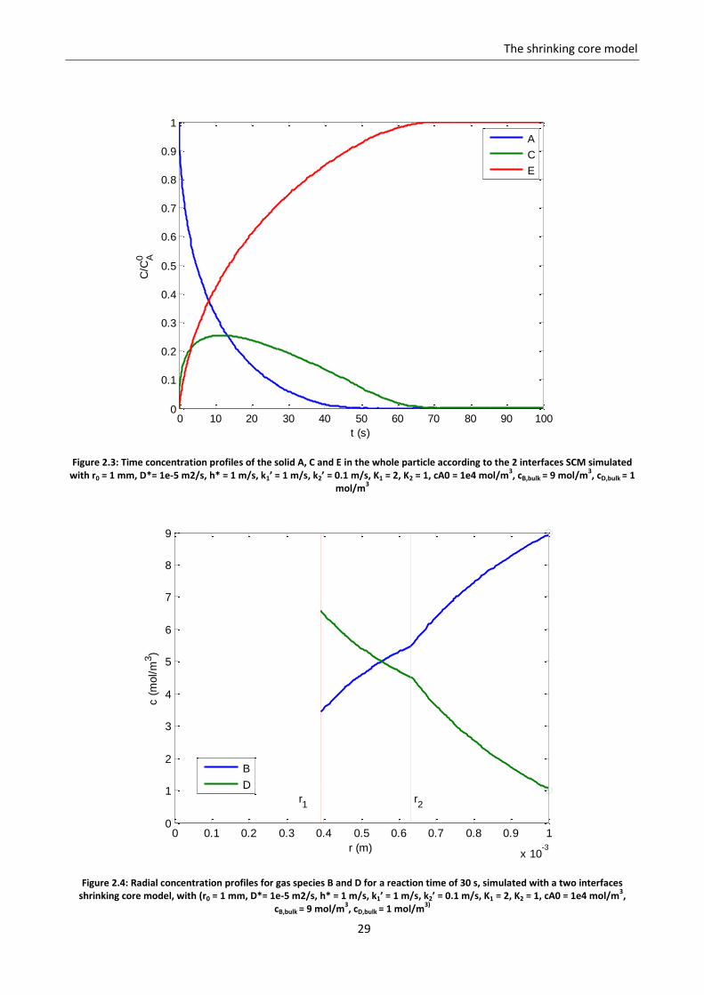
Figure 2.3 shows an example of the results of the model for the solid species for a given set of parameters
and operating conditions (r0 = 1 mm, D*= 1e-5 m2/s, h* = 1 m/s, k1’ = 1 m/s, k2’ = 0.1 m/s, K1 = 2, K2 = 1, cA0
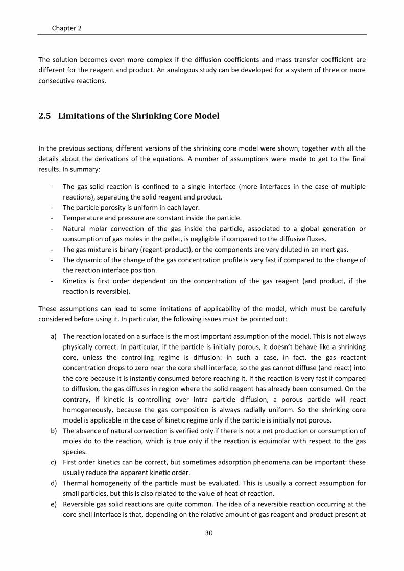
= 1e4 mol/m3, cB,bulk = 9 mol/m3, cD,bulk = 1 mol/m3). The results for the gas radial profiles are shown in figure
2.4 for a reaction time of 30 s.
The shrinking core model
29
Figure 2.3: Time concentration profiles of the solid A, C and E in the whole particle according to the 2 interfaces SCM simulated with r0 = 1 mm, D*= 1e-5 m2/s, h* = 1 m/s, k1’ = 1 m/s, k2’ = 0.1 m/s, K1 = 2, K2 = 1, cA0 = 1e4 mol/m
3, cB,bulk = 9 mol/m
3, cD,bulk = 1
mol/m3
Figure 2.4: Radial concentration profiles for gas species B and D for a reaction time of 30 s, simulated with a two interfaces shrinking core model, with (r0 = 1 mm, D*= 1e-5 m2/s, h* = 1 m/s, k1’ = 1 m/s, k2’ = 0.1 m/s, K1 = 2, K2 = 1, cA0 = 1e4 mol/m
3,
cB,bulk = 9 mol/m3, cD,bulk = 1 mol/m
3)
0 10 20 30 40 50 60 70 80 90 1000
0.1
0.2
0.3
0.4
0.5
0.6
0.7
0.8
0.9
1
t (s)
C/C
A0
A
C
E
0 0.1 0.2 0.3 0.4 0.5 0.6 0.7 0.8 0.9 1
x 10-3
0
1
2
3
4
5
6
7
8
9
r (m)
c (
mol/m
3)
B
D
r1 r
2
Chapter 2
30
The solution becomes even more complex if the diffusion coefficients and mass transfer coefficient are
different for the reagent and product. An analogous study can be developed for a system of three or more
consecutive reactions.
2.5 Limitations of the Shrinking Core Model
In the previous sections, different versions of the shrinking core model were shown, together with all the
details about the derivations of the equations. A number of assumptions were made to get to the final
results. In summary:
- The gas-solid reaction is confined to a single interface (more interfaces in the case of multiple
reactions), separating the solid reagent and product.
- The particle porosity is uniform in each layer.
- Temperature and pressure are constant inside the particle.
- Natural molar convection of the gas inside the particle, associated to a global generation or
consumption of gas moles in the pellet, is negligible if compared to the diffusive fluxes.
- The gas mixture is binary (regent-product), or the components are very diluted in an inert gas.
- The dynamic of the change of the gas concentration profile is very fast if compared to the change of
the reaction interface position.
- Kinetics is first order dependent on the concentration of the gas reagent (and product, if the
reaction is reversible).
These assumptions can lead to some limitations of applicability of the model, which must be carefully
considered before using it. In particular, the following issues must be pointed out:
a) The reaction located on a surface is the most important assumption of the model. This is not always
physically correct. In particular, if the particle is initially porous, it doesn’t behave like a shrinking
core, unless the controlling regime is diffusion: in such a case, in fact, the gas reactant
concentration drops to zero near the core shell interface, so the gas cannot diffuse (and react) into
the core because it is instantly consumed before reaching it. If the reaction is very fast if compared
to diffusion, the gas diffuses in region where the solid reagent has already been consumed. On the
contrary, if kinetic is controlling over intra particle diffusion, a porous particle will react
homogeneously, because the gas composition is always radially uniform. So the shrinking core
model is applicable in the case of kinetic regime only if the particle is initially not porous.
b) The absence of natural convection is verified only if there is not a net production or consumption of
moles do to the reaction, which is true only if the reaction is equimolar with respect to the gas
species.
c) First order kinetics can be correct, but sometimes adsorption phenomena can be important: these
usually reduce the apparent kinetic order.
d) Thermal homogeneity of the particle must be evaluated. This is usually a correct assumption for
small particles, but this is also related to the value of heat of reaction.
e) Reversible gas solid reactions are quite common. The idea of a reversible reaction occurring at the
core shell interface is that, depending on the relative amount of gas reagent and product present at
The shrinking core model
31
that interface, the interface can shift towards the particle centre or towards the external surface if
the reaction rate is globally positive or negative, respectively. This is not what happens, though. In
fact, the model always considers that the gas only diffuses through the solid product layer, without
reacting. If this is certainly true for the gas reagent, this cannot be true for the solid product, if the
reaction is reversible. In fact the solid product is a reagent for the gas product, so it must
necessarily react also in the layer. The core shell behavior could still be approximated for diffusive
regimes, because in these cases the gas product concentration is always maximum near the center
of the particle, where it is produced by the forward reaction that occurs because the solid reagent
concentration is higher. The core-shell assumption is however generally wrong for reversible
reactions.
f) For the same reason, multiple interfaces shrinking core are not physically possible. Again, in all the
layers between the core and the external shell, the gas is supposed to diffuse without reacting. But
the intermediate layers are actually made of solid phases that are not inert to the gas that is
moving through them. The model could be still correct for the case of very fast reactions (diffusive
regime). What happens in this case is that all the interfaces converge to a single radial coordinate,
and this also means that all the reaction steps take place simultaneously in a single point. In
summary, the particle behaves like a one interface shrinking core, where the only considered
reaction is the sum of all the reaction steps.
Despite these limitations, the shrinking core model is still widely used also for the more critical cases
considered, and several works with reversible and multi step reactions can be found in the literature. It is
still possible to make use of it, because of its simplicity and easy applicability to complex reactor problems.
Notation
a, b, c, d Reaction stoichiometric coefficients Biot number Local molar local concentration of i, total (mol/cm
3)
Total concentration of i inside the particle (mol/cm3)
Effective diffusion coefficient of i in j (cm2/s)
Effective diffusion coefficient of i in the solid phase k (cm
2/s)
Binary diffusion coefficient of i in j (cm2/s)
Damkohler number Mass transfer coefficient of i (cm/s) Molar diffusive flux of i (mol/cm
2/s)
Superficial kinetic constant (cm/s) Equilibrium constant Molecular weight of the core, of the i-th species (g/mol) Number of moles of reacting solid into the particle Number of moles of the i-th species into the particle N Total molar gas flux (mol/cm
2/s)
Radial coordinate (cm) Particle radius (cm)
Chapter 2
32
Radius of the core-shell interface (cm) R Reaction rate (mol/cm
3/s)
t Time (s) Volume of the core, of the i-th species (cm
3)
, Molar fraction of I, inside the particle, in the gas bulk phase
Particle conversion Greek letters ԑ Porosity Size change factor Density of the core, of the i-th species (g/cm
3)
Tortuosity Characteristic times of kinetic, diffusive, and external mass transfer resistances
33
Chapter 3. Application of SCM: Simulation of full scale reactors for Direct
Reduction of Iron
In chapter §2, the different formulations of the shrinking core model have been presented. Despite its
possible limitations, already discussed, the SCM is a simple approach to the description of gas solid
reactions, that can be successfully applied to describe full scale reactors. In particular, the SCM can be used
when a system of solid particles and gas is represented by a fully Eulerian approach: this implies that the
single particles are not tracked, but the gas-solid system is seen as a medium, and in any point of the
reactor the characteristics of the two phases (velocity field, composition and temperature) are quantified.
This is possible because the shrinking core model expresses the reaction rate of the whole particle as a
function of the global particle conversion and gas composition outside the particle, so no information is
needed about the local composition of the solid phases and diffusing gas inside the pellet itself. This also
means that the form of the reaction rates does not depend on the history of the reaction of the single
particle, but just on the current value of its degree of conversion, that automatically defines the
distribution of the solid phases into the particle.
In this chapter, an application of the SCM is presented. A 2D axial symmetric model of a DRP (direct
reduction plant) shaft furnace that includes momentum, species and enthalpy balances for the solid and
the gas phases was solved. The process consists in the reduction of iron ore pellets with H2 and CO mixtures
at high temperature. The process gas can contain natural gas, which is catalytically converted on metallic
iron by steam reforming and cracking reactions into syngas and carbon. This work was made thanks to the
collaboration to an industrial research project between the University of Padova and Centro Ricerche
Danieli. The industrial partner provided the data from real plants and dedicated pilot plants to fully
characterize the necessary kinetic parameters. The model was developed by means of a commercial CFD
code (Comsol Multiphisics [22]), that was occasionally coupled with an optimization routine in Matlab [23],
in order to fit the parameters of the SCM. The details of this work are reported in the next section [24].
3.1 Model overview
As a first step, a mathematical model was used to simulate the flow field of a granular material inside a silo.
The 2D axial-symmetric model was validated through a small scale (1:15) experimental reactor and it is able
to reproduce the flow and pressure fields of the solid [25]. This study assessed that, if the fluidization index
is well below unity, the influence of the gas flow field into the solid velocity is negligible and the calculation
of the solid flow field can be performed only once and then kept constant in the solution of the other
variables (gas flow field and temperature and composition profiles of both gas and solid), unless solid flow
rate is changed. Moreover, the solids velocity profile in the cylindrical zone is quite uniform, except in the
narrow shearing layer close to the wall.
Chapter 3
34
In this work the model of the continuous shaft reactor was developed with the introduction of the chemical
reactions between the gas and the solid and the addition of the energy balances for both phases. This
allowed the prediction of composition and temperature distribution, both for the solid and the gas. Similar
works, in 1D or 3D, which describe other direct reduction processes, are included in references [18, 26, 27].
None of those models describes the local velocity of the dense granular bed, always assuming plug flow,
with no attrition on the reactor walls, disregarding geometric singularities such as flow feeders and reactor
shape variations. Regarding the gas phase, when methane is among the reactants in the feed gas, these
models do not account for the methane chemistry, i.e. cracking and reforming, which instead is proven to
have great influence on the reduction kinetics [28]. The present study is originated by a tangible need to
gain more insight in the industrial process and to understand the effect of any action taken by the control
unit of the plant.
3.2 Mathematical model used in CFD
The granular material is treated as a non-Newtonian continuum fluid. In this method the viscosity of the
pseudo fluid is a function of a scalar called granular temperature, which is influenced by the flow profiles
and the interparticle contacts. At the wall a “slip length” is implemented, which allows reproducing
correctly the interactions between the shearing solid bed and the wall (e.g. boundary layer behavior).
The gas flow field is described by the Brinkman equation, a momentum balance suitable to represent a gas
flowing through a porous bed, and by a continuity equation that accounts for the mass
generation/consumption in the single phase due to the multiphase reaction between solids and gas.
The reduction reactions involve a solid species and a gas species. The iron ore, whose iron oxide is primarily
hematite, Fe2O3, is reduced progressively to magnetite (Fe3O4), wüstite (FeO) and iron (Fe) in three steps.
The ore contains some gangue, as well, which is assumed to be an inert in the reduction process. Since the
reaction from hematite to magnetite is very fast if compared to the other steps, only two steps, i.e. the
reduction from hematite to wüstite and from wüstite to iron, are considered, both with hydrogen and
carbon monoxide. Reactions from wüstite to iron are considered reversible and linked to the
thermodynamic equilibrium FeO/Fe.
R1,H2: Fe2O3 + H2 → 2FeO + H2O ΔHR,298 = 46.6 kJ/mol
3.1
R1,CO: Fe2O3 + CO → 2FeO + CO2 ΔHR,298 = 5.49 kJ/mol
3.2
R2,H2: FeO + H2 Fe + H2O ΔHR,298 = 25.5 kJ/mol
3.3
R2,CO: FeO + CO Fe + CO2 ΔHR,298 = −15.7 kJ/mol
3.4
The species production/consumption rates are based on the shrinking core model, in the form of the two
interfaces formulation reported in chapter §2. The parameters of the model were taken both from
literature [29, 30] and from internal data coming from the ENERGIRON plants (developed by Tenova and
Danieli). Furthermore, an experimental campaign was held in Danieli R&D, where a semi-batch reactor with
Application of SCM: Simulation of full scale reactors for Direct Reduction of Iron
35
a capacity of 2 kg of iron ore and fed with the same process gas as in the industrial plant, working up to 12
bar gauge and 1100°C, was installed. Gas diffusivities in solids increase from hematite to wüstite and from
wüstite to sponge iron, with internal porosity varying from a 20% of hematite to 60-70% of sponge iron
[31]. As reported in literature [28], the carbon deposited on the pellet puts another barrier to diffusion and
slows down the reactions, both the catalytic and the reduction ones. Therefore, the reaction rates are
multiplied by a reducing factor accounting for the local amount of carbon.
Reducing gas (RG), rich in H2, CO and CH4, coming in contact with metallic iron, participates to the catalytic
reactions:
Steam Reforming, RSR: CH4 + H2O CO + 3H2 ΔHR,298 = 206.9 kJ/mol
3.5
Water Gas Shift, RW: CO + H2O CO2 + H2 ΔHR,298 = −41.16 kJ/mol
3.6
Methane Cracking, RC: CH4 → CS + 2H2 ΔHR,298 = 75.5 kJ/mol
3.7
Coke Gasification, RG: CS + H2O → CO + H2 ΔHR,298 = 131.4 kJ/mol
3.8
In addition to the species conservation equation, for both solid and gas phases, the energy balances are
solved including conductive heat losses from the reactor walls.
3.3 Model results
The main advantage of this model is the coupling between the flow field of solid and gas and the kinetic
and thermal equations. There are several gas streams entering the reactor in different positions without
mixing and influencing the internal macro-structure, i.e. the mapping of the different zones wetted by a
particular gas.
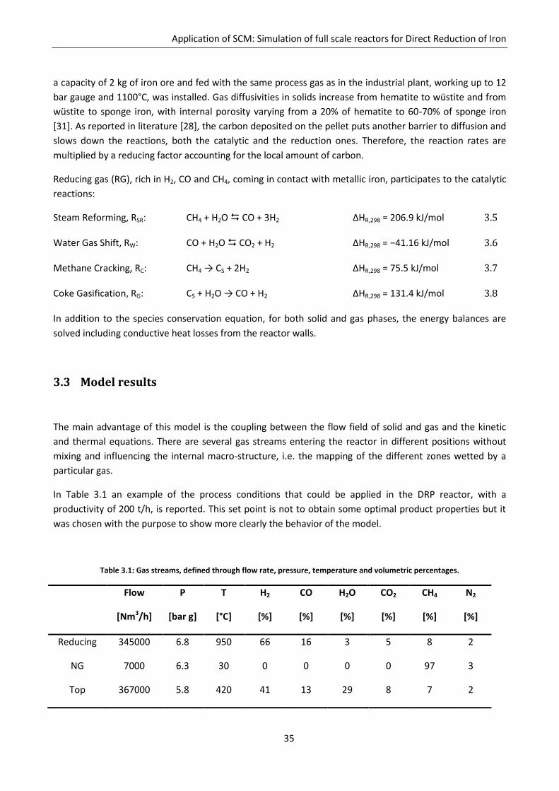
In Table 3.1 an example of the process conditions that could be applied in the DRP reactor, with a
productivity of 200 t/h, is reported. This set point is not to obtain some optimal product properties but it
was chosen with the purpose to show more clearly the behavior of the model.
Table 3.1: Gas streams, defined through flow rate, pressure, temperature and volumetric percentages.
Flow
[Nm3/h]
P
[bar g]
T
[°C]
H2
[%]
CO
[%]
H2O
[%]
CO2
[%]
CH4
[%]
N2
[%]
Reducing
NG
Top
345000
7000
367000
6.8
6.3
5.8
950
30
420
66
0
41
16
0
13
3
0
29
5
0
8
8
97
7
2
3
2
Chapter 3
36
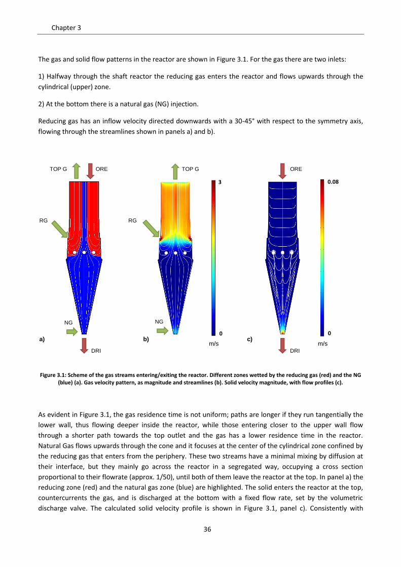
The gas and solid flow patterns in the reactor are shown in Figure 3.1. For the gas there are two inlets:
1) Halfway through the shaft reactor the reducing gas enters the reactor and flows upwards through the
cylindrical (upper) zone.
2) At the bottom there is a natural gas (NG) injection.
Reducing gas has an inflow velocity directed downwards with a 30-45° with respect to the symmetry axis,
flowing through the streamlines shown in panels a) and b).
Figure 3.1: Scheme of the gas streams entering/exiting the reactor. Different zones wetted by the reducing gas (red) and the NG (blue) (a). Gas velocity pattern, as magnitude and streamlines (b). Solid velocity magnitude, with flow profiles (c).
As evident in Figure 3.1, the gas residence time is not uniform; paths are longer if they run tangentially the
lower wall, thus flowing deeper inside the reactor, while those entering closer to the upper wall flow
through a shorter path towards the top outlet and the gas has a lower residence time in the reactor.
Natural Gas flows upwards through the cone and it focuses at the center of the cylindrical zone confined by
the reducing gas that enters from the periphery. These two streams have a minimal mixing by diffusion at
their interface, but they mainly go across the reactor in a segregated way, occupying a cross section
proportional to their flowrate (approx. 1/50), until both of them leave the reactor at the top. In panel a) the
reducing zone (red) and the natural gas zone (blue) are highlighted. The solid enters the reactor at the top,
countercurrents the gas, and is discharged at the bottom with a fixed flow rate, set by the volumetric
discharge valve. The calculated solid velocity profile is shown in Figure 3.1, panel c). Consistently with
TOP G ORE TOP G ORE
RG RG
a) b) c)
DRI DRI
NG NG
m/s m/s
3
0
0.08
0
Application of SCM: Simulation of full scale reactors for Direct Reduction of Iron
37
previous experiments [25], in the cylindrical zone a plug flow prevails in most of the cross section (Figure
3.1 c). However, flow modifications determined by the flow feeders are correctly predicted.
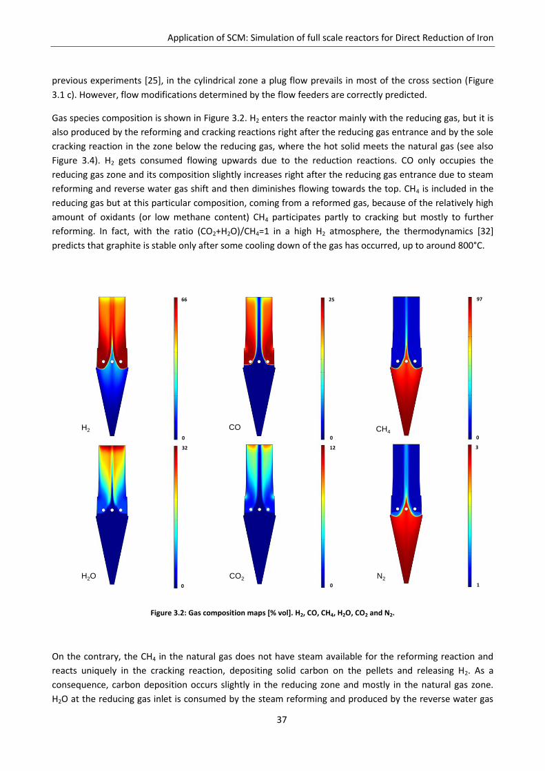
Gas species composition is shown in Figure 3.2. H2 enters the reactor mainly with the reducing gas, but it is
also produced by the reforming and cracking reactions right after the reducing gas entrance and by the sole
cracking reaction in the zone below the reducing gas, where the hot solid meets the natural gas (see also
Figure 3.4). H2 gets consumed flowing upwards due to the reduction reactions. CO only occupies the
reducing gas zone and its composition slightly increases right after the reducing gas entrance due to steam
reforming and reverse water gas shift and then diminishes flowing towards the top. CH4 is included in the
reducing gas but at this particular composition, coming from a reformed gas, because of the relatively high
amount of oxidants (or low methane content) CH4 participates partly to cracking but mostly to further
reforming. In fact, with the ratio (CO2+H2O)/CH4=1 in a high H2 atmosphere, the thermodynamics [32]
predicts that graphite is stable only after some cooling down of the gas has occurred, up to around 800°C.
Figure 3.2: Gas composition maps [% vol]. H2, CO, CH4, H2O, CO2 and N2.
On the contrary, the CH4 in the natural gas does not have steam available for the reforming reaction and
reacts uniquely in the cracking reaction, depositing solid carbon on the pellets and releasing H2. As a
consequence, carbon deposition occurs slightly in the reducing zone and mostly in the natural gas zone.
H2O at the reducing gas inlet is consumed by the steam reforming and produced by the reverse water gas
H2 CO CH4
H2O CO2 N2
66
0
25
0 0
97
0
32 12
0
3
1
Chapter 3
38
shift. Further on, steam is produced more abundantly by the reduction reactions in the cylindrical zone and
in very little extent in the conical zone. CO2 is consumed by the reverse water gas shift reaction (the model
does not account for dry reforming) and then produced, but only in the zone occupied by the reducing gas,
complementarily to CO.
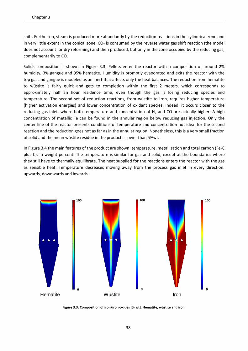
Solids composition is shown in Figure 3.3. Pellets enter the reactor with a composition of around 2%
humidity, 3% gangue and 95% hematite. Humidity is promptly evaporated and exits the reactor with the
top gas and gangue is modeled as an inert that affects only the heat balances. The reduction from hematite
to wüstite is fairly quick and gets to completion within the first 2 meters, which corresponds to
approximately half an hour residence time, even though the gas is losing reducing species and
temperature. The second set of reduction reactions, from wüstite to iron, requires higher temperature
(higher activation energies) and lower concentration of oxidant species. Indeed, it occurs closer to the
reducing gas inlet, where both temperature and concentration of H2 and CO are actually higher. A high
concentration of metallic Fe can be found in the annular region below reducing gas injection. Only the
center line of the reactor presents conditions of temperature and concentration not ideal for the second
reaction and the reduction goes not as far as in the annular region. Nonetheless, this is a very small fraction
of solid and the mean wüstite residue in the product is lower than 5%wt.
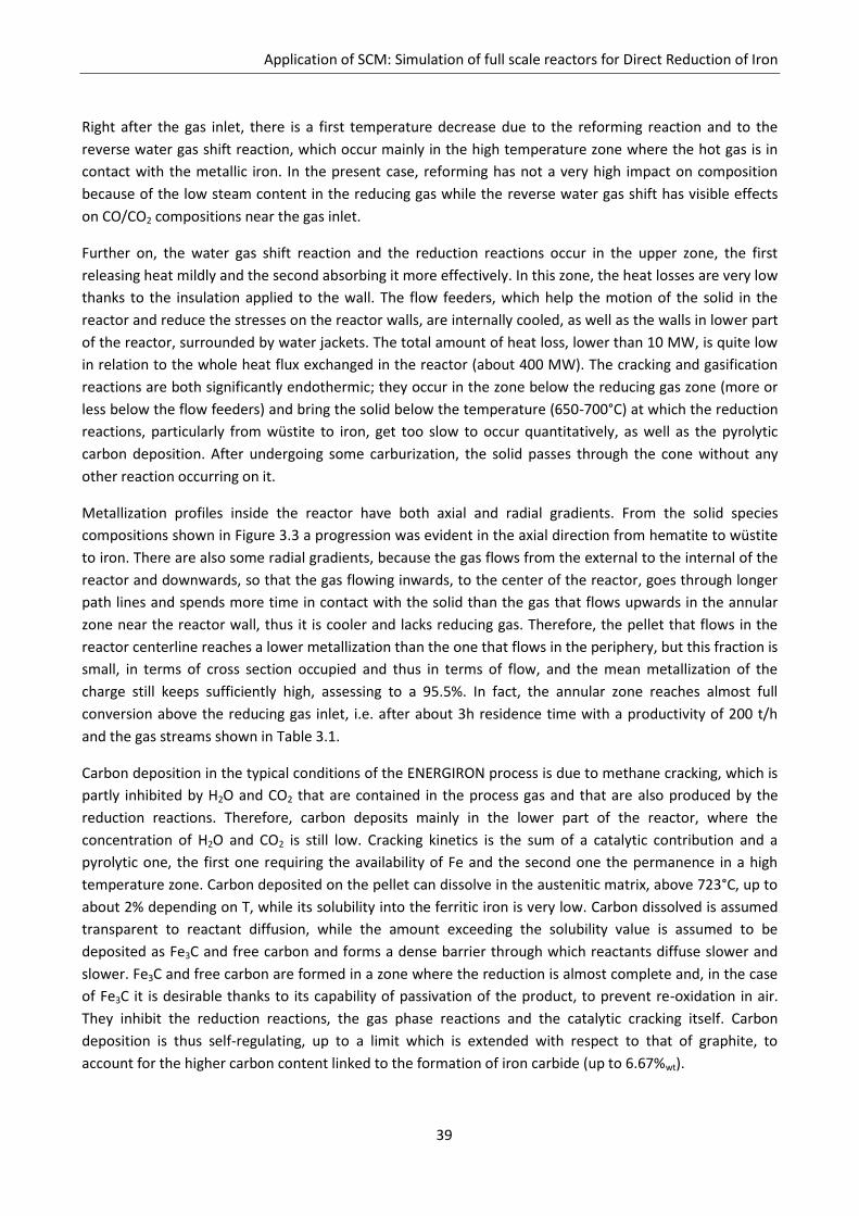
In Figure 3.4 the main features of the product are shown: temperature, metallization and total carbon (Fe3C
plus C), in weight percent. The temperature is similar for gas and solid, except at the boundaries where
they still have to thermally equilibrate. The heat supplied for the reactions enters the reactor with the gas
as sensible heat. Temperature decreases moving away from the process gas inlet in every direction:
upwards, downwards and inwards.
Figure 3.3: Composition of iron/iron-oxides [% wt]. Hematite, wüstite and iron.
Hematite Wüstite Iron0
100
0 0
100 100
Application of SCM: Simulation of full scale reactors for Direct Reduction of Iron
39
Right after the gas inlet, there is a first temperature decrease due to the reforming reaction and to the
reverse water gas shift reaction, which occur mainly in the high temperature zone where the hot gas is in
contact with the metallic iron. In the present case, reforming has not a very high impact on composition
because of the low steam content in the reducing gas while the reverse water gas shift has visible effects
on CO/CO2 compositions near the gas inlet.
Further on, the water gas shift reaction and the reduction reactions occur in the upper zone, the first
releasing heat mildly and the second absorbing it more effectively. In this zone, the heat losses are very low
thanks to the insulation applied to the wall. The flow feeders, which help the motion of the solid in the
reactor and reduce the stresses on the reactor walls, are internally cooled, as well as the walls in lower part
of the reactor, surrounded by water jackets. The total amount of heat loss, lower than 10 MW, is quite low
in relation to the whole heat flux exchanged in the reactor (about 400 MW). The cracking and gasification
reactions are both significantly endothermic; they occur in the zone below the reducing gas zone (more or
less below the flow feeders) and bring the solid below the temperature (650-700°C) at which the reduction
reactions, particularly from wüstite to iron, get too slow to occur quantitatively, as well as the pyrolytic
carbon deposition. After undergoing some carburization, the solid passes through the cone without any
other reaction occurring on it.
Metallization profiles inside the reactor have both axial and radial gradients. From the solid species
compositions shown in Figure 3.3 a progression was evident in the axial direction from hematite to wüstite
to iron. There are also some radial gradients, because the gas flows from the external to the internal of the
reactor and downwards, so that the gas flowing inwards, to the center of the reactor, goes through longer
path lines and spends more time in contact with the solid than the gas that flows upwards in the annular
zone near the reactor wall, thus it is cooler and lacks reducing gas. Therefore, the pellet that flows in the
reactor centerline reaches a lower metallization than the one that flows in the periphery, but this fraction is
small, in terms of cross section occupied and thus in terms of flow, and the mean metallization of the
charge still keeps sufficiently high, assessing to a 95.5%. In fact, the annular zone reaches almost full
conversion above the reducing gas inlet, i.e. after about 3h residence time with a productivity of 200 t/h
and the gas streams shown in Table 3.1.
Carbon deposition in the typical conditions of the ENERGIRON process is due to methane cracking, which is
partly inhibited by H2O and CO2 that are contained in the process gas and that are also produced by the
reduction reactions. Therefore, carbon deposits mainly in the lower part of the reactor, where the
concentration of H2O and CO2 is still low. Cracking kinetics is the sum of a catalytic contribution and a
pyrolytic one, the first one requiring the availability of Fe and the second one the permanence in a high
temperature zone. Carbon deposited on the pellet can dissolve in the austenitic matrix, above 723°C, up to
about 2% depending on T, while its solubility into the ferritic iron is very low. Carbon dissolved is assumed
transparent to reactant diffusion, while the amount exceeding the solubility value is assumed to be
deposited as Fe3C and free carbon and forms a dense barrier through which reactants diffuse slower and
slower. Fe3C and free carbon are formed in a zone where the reduction is almost complete and, in the case
of Fe3C it is desirable thanks to its capability of passivation of the product, to prevent re-oxidation in air.
They inhibit the reduction reactions, the gas phase reactions and the catalytic cracking itself. Carbon
deposition is thus self-regulating, up to a limit which is extended with respect to that of graphite, to
account for the higher carbon content linked to the formation of iron carbide (up to 6.67%wt).
Chapter 3
40
Figure 3.4: Maps of solid carbon, metallization and temperature. The carbon map contains the contour (in white) of the region
where carbon is deposited.
Results thus indicate several interactions between the local status (velocity, composition and temperature)
and the reactions:
1) Carbon that forms in the lower part of the reactor is a further diffusion resistance for the reactants.
2) Nonetheless, oxidant species (H2O and CO2) intervene in the thermodynamic equilibrium of
graphite/Fe3C, preventing or decelerating the cracking of methane.
3) Metallic iron is a requisite to have catalytic activity in the reforming and catalytic cracking reactions.
4) High temperature is required to have pyrolytic cracking, gasification, steam reforming and, to a lesser
extent, reduction of wüstite.
5) Cracking and mainly steam reforming are highly endothermic and strongly affect the temperature map
inside the reactor.
6) Carbon dissolved in the iron matrix (thus not blocking the diffusion of reactants) depends on
temperature.
3.4 Conclusions
A 2D axial symmetric model of the DRP shaft reactor has been developed to study the internal behavior of
the reactor. Reduction and gas phase reactions were included in the model, as well as the complex
Application of SCM: Simulation of full scale reactors for Direct Reduction of Iron
41
interactions between the species (gas and solid) distribution and the kinetics. Simulations put in evidence
the following main features:
- The flow field inside the reactor is calculated, both for solid and for gas, and the relative contact time is
evaluated, evidencing different zones of wetting which can more or less favor the reduction reactions.
- The map of temperature is determined by and in turns determines the kinetics of the reactions occurring
in the shaft reactor, where the only heat is supplied by the process gas. Consistent modeling of the local
heat fluxes is crucial.
- Gas and solid compositions together with the kinetics of reduction and cracking where localized and
characterized, in a complex net of interconnections that enhance or restrain the reduction and
carburization of the product. In particular, it was understood that the chemistry of methane is the
uppermost factor influencing the performances of the shaft reactor: temperature, metallization and
especially carbon deposition.
The simulation model allows gaining a fundamental understanding of the major phenomena that intervene
in determining the measured temperature, metallization and carburization of the DRI. The model will be
used as a tool for choosing the optimum operation set points in terms of metallization, carbon content and
energy consumption of the process.

Chapter 3
42
43
Chapter 4. Continuous Models
In the previous sections, details about shrinking core models and their possible applicability have been
discussed. SCM can in some cases be successfully used to describe non catalytic gas solid reaction
processes, when its limitations are taken into account. For a more accurate description of a gas solid
reacting system, a continuous model must be used.
4.1 Material balances
In SCM the reaction is assumed to take place only on a surface, fully characterized by a coordinate within
the pellet. On the contrary, continuous models assume that the gas solid reaction can take place in any
point of the particle, together with gas transport phenomena. The gas concentration transport inside the
particle is ruled by the chemical species conservation equation:
4.1
In this formulation,
is the molar concentration of gas species i, is the local particle porosity,
is the
molar flux of i, and is the source term, associated with the reaction. The local porosity is defined as the
ratio between the volume occupied by the gas and the total volume (gas + solid). It can vary both in space
and time for effect of the reaction and physical phenomena related to the change of the solid structure (for
instance sintering, particle shrinking or swelling). The porosity term is present in the time derivative
because in equation 4.1,
is defined as the number of moles of i per unit of volume of gas, whereas the
global equation is expressed in terms of variation of number of moles per unit of total volume. The molar
flux of i can be expressed as the sum of a convective and a diffusive part:
4.2
Where
is the molar fraction of i, is the total molar gas flux, and is the molar diffusive flux of i. The
advantage of using this formulation is that can be expressed as a function of the gradient of
concentration of the gas species, thanks to Fick’s law or multicomponent diffusion models. This part will be
discussed in detail in section 5. The total molar flux can be instead calculated by the total concentration
balance:
4.3
Chapter 4
44
In this formulation, c is the total gas concentration. Since it is expressed per unit of volume of gas, it can be
directly calculated through an equation of state, for instance the ideal gas law:
4.4
Equation 4.3 derives from the sum of all equations 4.1 expressed for every gas species. The total gas flux is
in fact equal to the sum of the convective fluxes of all species, whereas the sum of all diffusive fluxes is
always zero by definition. Equation 4.3 describes the total conservation of mass in gas phase in terms of
number of moles. Since the total gas concentration is already expressed by equation 4.4, equation 4.3 can
be solved in the divergence of . For the solid phase, the concentration balance for the i-th species can be
expressed by:
4.5
In this equation, porosity is not present in the time derivative, because is expressed as the concentration
of the solid i per unit of total volume (otherwise a factor 1-ε should be included). The total molar flux of
solid can be associated to a local shrinking or swelling of the solid.
A total concentration balance can also be expressed for the solid phase, by summing all of the balances for
the solid species:
4.6
Where is the local concentration of solid phase. Differently from what previously stated for equation 4.3,
no equation of state can be used to determine , so equation 4.6 cannot be solved in terms of unless
another equation is found to express or its variation in time. It’s not trivial to understand the physical
meaning of the left hand side of equation 4.6, but it can be actually related to the variation of the local
porosity in time. Using the definition of local porosity we obtain:
4.7
Where is the volume occupied by the solid phase, and V is the total volume. By multiplying the ratio in
equation 4.7 by the total number of moles of solid, , we get:
4.8
Where we recognized that the ratio between the total number of solid moles and the total volume is equal
to , by definition. The total volume of solid can be expressed as the sum of the volumes occupied by the
single solid species, considering the dense materials:
Continuous Models
45
4.9
Where and are the molecular weight and the intrinsic density of the j-th solid species, respectively.
The intrinsic density is a constant property of the dense material, and only depends on the type of atoms
forming the chemical species, and its crystal structure. By using equation 4.9 into 4.8, the equation of
porosity becomes:
4.10
This equation relates the porosity to the total solid concentration. Taking the derivative of equation 4.10 in
time, we obtain:
4.11
Finally, using the equation for the single solid species 4.5 into 4.11, we obtain the equation of conservation
of total mass for the solid phase, written in terms of porosity:
4.12
This equation states that the variations of porosity in time may be due either to a local effect of shrinking or
swelling of the particle (terms associated to the divergence of ), or to the change of composition
caused by chemical reaction, involving species with different intrinsic densities (terms associated with the
source factors ).
The source terms for both the gas and solid balances are a function of the reaction rates:
4.13
4.14
Where
and are the stoichiometric coefficients of the i-th gas species and i-th solid species in the
reaction j, respectively.
Chapter 4
46
4.2 Energy balance
A heat production or consumption is generally associated with the chemical reactions within the particle.
An energy balance must be included in the model in order to characterize the temperature in any point of
the particle. This can be estimated, considering a single pseudo phase made of both solid and gas, by
starting from the equation of transport of total enthalpy in the system:
4.15
In this equation, is the total enthalpy of the system per unit of total volume, is the total flux of
enthalpy associated with convection, and is the total flux associated with thermal conduction. These
quantities can be expressed as a function of the properties of the two phases, solid and gas, composing the
medium. In particular:
4.16
Where is the enthalpy of gas per unit of mole of gas mixture and is the enthalpy of solid per unit of
mole of solid mixture. A porosity factor is present in the gas part, because the total gas concentration is
defined with respect to the volume of gas whereas the total solid concentration as a function of the total
volume. The total convective flux of enthalpy is:
4.17
The conductive flux can be expressed through the Fourier law, considering a pseudo conductivity of the
medium, weighted on the relative amount of occupied volume:
4.18
Where and are the conductivities of the gas and solid phases, respectively. They can be calculated
using a rule of mixtures, as the one reported:
4.19
4.20
Equation 4.15 becomes, making use of 4.16-4.18:
4.21
Continuous Models
47
The total enthalpies of gas and solid phase can be expressed through a simple rule of mixture, neglecting
the enthalpies of mixing. So, for instance, for the gas:
4.22
The derivatives in the differential equation 4.21 can be decomposed as a function of the phases
compositions and temperature, making use of the definition of heat capacity:
4.23
Consistently with the units used so far, this heat capacity is defined on a molar base (J/mol/K or its
multiples).
The accumulation term relative to the gas phase can be decomposed as follows:
4.24
The same rule of mixtures of the enthalpy can be applied to the heat capacity of the gas, phase:
4.25
So equation 4.24 becomes:
4.26
The same mathematical procedure can be applied to the convective part, obtaining:
4.27
By summing equations 4.26 and 4.27, we obtain:
4.28
It can be immediately recognized that the factors in the sum in equation 4.28 can be expressed by making
use of the equation of conservation of the single gas species (4.1 and 4.3), so that:
Chapter 4
48
4.29
For the solid phase we can get to a similar result:
4.30
Equations 4.29 and 4.30 can be used in equation 4.21, obtaining equation 4.31:
4.31
In equation 4.31, the two sums of the source terms have been collected in a single sum, related to all the
species (solid + gas). That term source term can be further developed, by using equations 4.13-4.14, and
recalling the definition of heat of reaction:
4.32
The final result for the energy balance is:
4.33
This final form shows in a better way the relationship between the temperature changes inside the gas-
solid medium and the different mechanisms of transport of mass and energy. In particular, temperature
changes may be due to:
- Transport of energy associated with the convective flux of gas .
- Transport of energy associated with the convective flux of solid .
- Transport of energy associated with the diffusive fluxes of gas species .
- Transport of energy by conduction in both solid and gas phases.
- Heat production generated by the chemical reactions .
In common practice, when describing the energy transport in porous solids, the first and third contributions
are neglected. A simplified version of equation 4.33 is used instead, which is:
4.34
Continuous Models
49
Where the global heat capacity and conductivity are:
4.35
4.36
In general, a number of parameter are temperature dependent in the energy balance ( , , , ,
,
, ).
4.3 Model for spherical particles
According to the continuous model described so far, the evolution of the gas-solid medium can be
described through the system of equations 4.1, 4.3, 4.5, 4.6, 4.10 and 4.33 (possibly replaced by 4.34). The
variables to solve are
, , , , , P, T. Considering that the total fluxes have generally three
components for a 3D system, the number of equations is not sufficient to determine the solution. For the
gas phase, a momentum balance could be added. In this sense, the Darcy equation is usually a good choice:
this relates the gas pressure gradient with the gas velocity field, through the viscosity and permeability
parameters. Once the velocity field is calculated, the molar flux can be found by scaling it by the total gas
concentration.
Usually, the continuous model dimensionality can be simplified, thanks to the symmetric behavior of the
described geometry. For the case of solid spherical particles, if the boundary and initial conditions applied
to the system are homogeneous along the angular coordinates, the presented model can be reduced to a
mono dimensional one, where only the radial components of the gradients and divergences are taken into
account. The equations of conservation of the gas and solid species, and the energy balance become,
according to this simplifications:
4.37
4.38
4.39
4.40
4.41
Chapter 4
50
In this formulation, and are the radial components of the total molar fluxes of gas and solid,
respectively, while is the radial component of the diffusive flux of the i-th gas species. These five
equations must be added to the equation of porosity (4.10), the gas equation of state (4.4), and the
equations for the production rates (4.13-4.14). Besides, a diffusion model is needed to express and a
kinetic model is needed to express . These will be discussed further on. Usually the value of the gas
pressure P can be assumed to be radially constant. If this is true, no momentum equation is needed, and
the total molar flux of gas can be calculated from the total concentration equation (4.8). In fact, this
becomes:
4.42
Where the time derivative of porosity can be expressed through equation 4.11 and the time derivative of
temperature through equation 4.41.
The system still needs a closure to determine the solid flux . Nevertheless, in most application the effect
of change in size of the particle can be neglected. If this is true, can be assumed to be zero. The
equation of conservation of the solid species and total solid concentration become:
4.43
4.44
In this formulation, no spatial derivatives are present in the equations for the solid. It’s important to point
out that this does not imply that and only change in time and are constant in r, because the terms
will necessarily depend on the concentration of the gas species, which are generally different in any radial
coordinate because the spatial derivatives in equations 4.37-4.38 are still present. The equation that
describes the evolution of the porosity, according to the constant volume assumption becomes:
4.45
Finally, the equation for the total gas flux becomes:
4.46
This equation states that a total molar gas flux can be generated by these following phenomena:
- Chemical reactions with solid reagents and products having different densities and molecular
weights.
Continuous Models
51
- Radial gradients of temperature.
- Chemical reactions with nonzero net heat production.
- Chemical reactions with a net production of number of gas moles.
The first three phenomena are present in almost every case, whereas in some situations the gas solid
reactions are equimolar with respect to the gas species, in which case the last sum of the right hand side of
equation 4.46 is zero. From a different point of view, the terms related to the first three phenomena are
usually of little importance in equation 4.46: in fact, in many cases the radial gradients are small and the
particle temperature can be considered as more or less uniform, and the first sum in the right hand side of
equation 4.46 is small. On the contrary the net production of gas moles can be important for non equimolar
reactions.
4.4 Boundary and initial conditions
The system of partial differential equations obtained by the previous analysis can be solved, once a proper
set of boundary and initial conditions is provided. For equations 4.37and 4.41, two boundary conditions are
needed, whereas for equations 4.38, 4.39 and 4.40 only one is necessary. At the centre of the particle (r =
0), symmetry conditions must be used: in particular, all fluxes must be zero, otherwise a net production of
mass or energy is created. This is equal to assume that the radial derivatives of all the variables are equal to
zero.
4.47
If equation 4.43 and 4.44 are used to describe the solid phase, no boundary conditions are needed from a
mathematical point of view. However, the solid concentration profiles will implicitly satisfy a condition of
zero derivative at the centre of the particle, that derives from the source term which is function of the gas
concentration profile where that boundary condition is applied. At the external particle surface, r = r0, the
gas composition and temperature may be known, if no external mass and energy resistances are present: in
such a case, a Dirichlet boundary condition can be used:
4.48
Where and are the concentration of the i-th gas species and temperature at the bulk,
respectively. This condition is usually true if the gas velocity is high outside the particle, so that convection
can overcome the concentration gradients near the particle surface that naturally arise because of reaction.
Chapter 4
52
If these gradients are still important,
and are generally different from the bulk values. In this situation,
a condition on the fluxes is applied at the boundary, using the heat and mass transfer coefficient approach:
4.49
Equations 4.49 state that the mass and energy fluxes approaching the particle surface from the inside must
be equal to the ones calculated approaching from the outside. In this formulation, and are the mass
transfer coefficient of the i-th species and the heat transfer coefficient, respectively. This approach allows
not to model the transport phenomena outside the particle in detail, which will necessarily imply a 2D or
3D approach, because the gas velocity field outside the particle is always too much complex to be described
with a monodimensional approach.
The initial conditions for the system are reported in equation 4.50:
4.50
Usually, uniform radial profiles are assumed at the beginning of reaction.
4.5 Reaction models
In the sets of equations presented so far, a kinetic model must be provided to characterize the values of the
reaction rates Rj as a function of the local gas and solid reagents, and temperature. A set of reactions can
be considered, in the following form:
4.51
Possible variations can consider solid or gas product, in which case the mathematical approach is very
similar to the one presented. The form of the reaction rate associated to the presented stoichiometry can
be expressed by the following general expression:
4.52
Where is the kinetic constant associated to the reaction,
and
are the concentrations of the gas
reagent and product, and is the conversion of the solid reagent, which is a function of the local
concentration if the solid reagent, as follows:
Continuous Models
53
4.53
The formulation in equation 4.51 separates the dependency on the three variables into the product of
three functions. The kinetic constant only depends on temperature, through the Arrhenius law:
4.54
Where A and Ea are the pre exponential factor and activation energy, respectively, and are characteristic of
the chemical reaction. The form of the functions f and g can be different, according to different models.
4.5.1 Effect of the gas concentration
The dependency on the gas concentration of the reaction rate is expressed through the function g. The
simplest approach is assuming a power law on the concentration of the reagent, that is:
4.55
Where β is a parameter, usually assumed equal to the stoichiometric coefficient b or equal to one. A more
complex function can be found, if an adsorption mechanism is included in the kinetic scheme. As a matter
of fact, all gas-solid reactions are superficial, and the gas species must reach the solid phase before
reacting. The global reaction described by equation 4.51 can be decomposed for the gas part into a series
of elementary steps, as follows:
4.56
4.57
4.58
In such a formulation, S is the free solid site, and are the adsorbed species B and D. The adsorption
and desorption reactions of both B and D are taken into account. Assuming first order reaction for all of the
elementary steps, the reaction rates associated with them are as follows:
4.59
4.60
4.61
The quantities and are the fractions of solid surface occupied by the gas B and D, respectively,
while is the fraction of empty surface. The Langmuir-Hinshelwood approach allows finding an analytical
expression for R2 as a function of the concentrations of free gas alone. First of all, the pseudo steady state
approximation is applied to the production rates of , and , obtaining the equations:
Chapter 4
54
4.62
4.63
These two equations can be coupled with the equation of overall balance of the surface:
4.64 Equations 4.62-4.64 are a system of three equations that can be solved in the variables , and . A
further simplification can be used: if it is assumed that the step of equation 4.60 is slow if compared to the
other two, reactions 4.59 and 4.61 will be near equilibrium. This means that the reactions rates R1 and R3
are zero. The surface fractions occupied by and can then be calculated as a function of the fraction
of free surface, as follows:
4.65
4.66
Now, using equation 4.64, is found:
4.67
Combining this with equations 4.65 and 4.60 we obtain:
4.68
More simplifications can be introduced, depending on the equilibrium of adsorption and desorption. In
particular, it is trivial to prove that if both adsorption and desorption equilibria are shifted to the products
in reactions 4.56 and 4.58, then KA approaches infinite and KD approaches zero, which means that R2
becomes a first order expression in .
It’s important to point out that the Langmuir-Hinshelwood model was developed for catalysis problems,
where the reaction generally does not have an effect on the solid composition and structure of the solid
matrix. When the solid phase reacts, things are more complicated, because the reacting surface is changing
itself. So equation 4.68 cannot fully replace equation 4.52. On the other hand, the phenomena related to
the gas phase can still be described with the same approach. Equation 4.68 can then be used to express the
function g:
4.69
The parameters and may be also dependent from temperature.
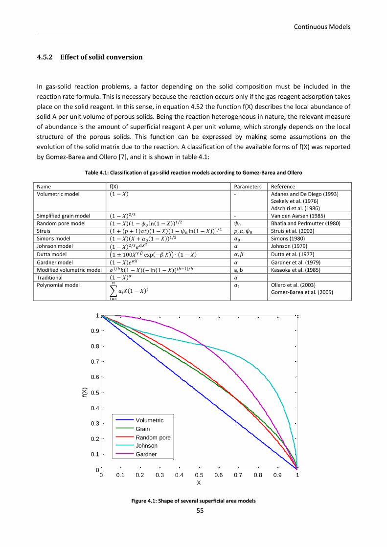
Continuous Models
55
4.5.2 Effect of solid conversion
In gas-solid reaction problems, a factor depending on the solid composition must be included in the
reaction rate formula. This is necessary because the reaction occurs only if the gas reagent adsorption takes
place on the solid reagent. In this sense, in equation 4.52 the function f(X) describes the local abundance of
solid A per unit volume of porous solids. Being the reaction heterogeneous in nature, the relevant measure
of abundance is the amount of superficial reagent A per unit volume, which strongly depends on the local
structure of the porous solids. This function can be expressed by making some assumptions on the
evolution of the solid matrix due to the reaction. A classification of the available forms of f(X) was reported
by Gomez-Barea and Ollero [7], and it is shown in table 4.1:
Table 4.1: Classification of gas-silid reaction models according to Gomez-Barea and Ollero
Name f(X) Parameters Reference
Volumetric model - Adanez and De Diego (1993) Szekely et al. (1976) Adschiri et al. (1986)
Simplified grain model - Van den Aarsen (1985)
Random pore model Bhatia and Perlmutter (1980)
Struis Struis et al. (2002)
Simons model Simons (1980)
Johnson model Johnson (1979)
Dutta model Dutta et al. (1977)
Gardner model Gardner et al. (1979)
Modified volumetric model a, b Kasaoka et al. (1985)
Traditional
Polynomial model
Ollero et al. (2003)
Gomez-Barea et al. (2005)
Figure 4.1: Shape of several superficial area models
0 0.1 0.2 0.3 0.4 0.5 0.6 0.7 0.8 0.9 10
0.1
0.2
0.3
0.4
0.5
0.6
0.7
0.8
0.9
1
X
f(X
)
Volumetric
Grain
Random pore
Johnson
Gardner
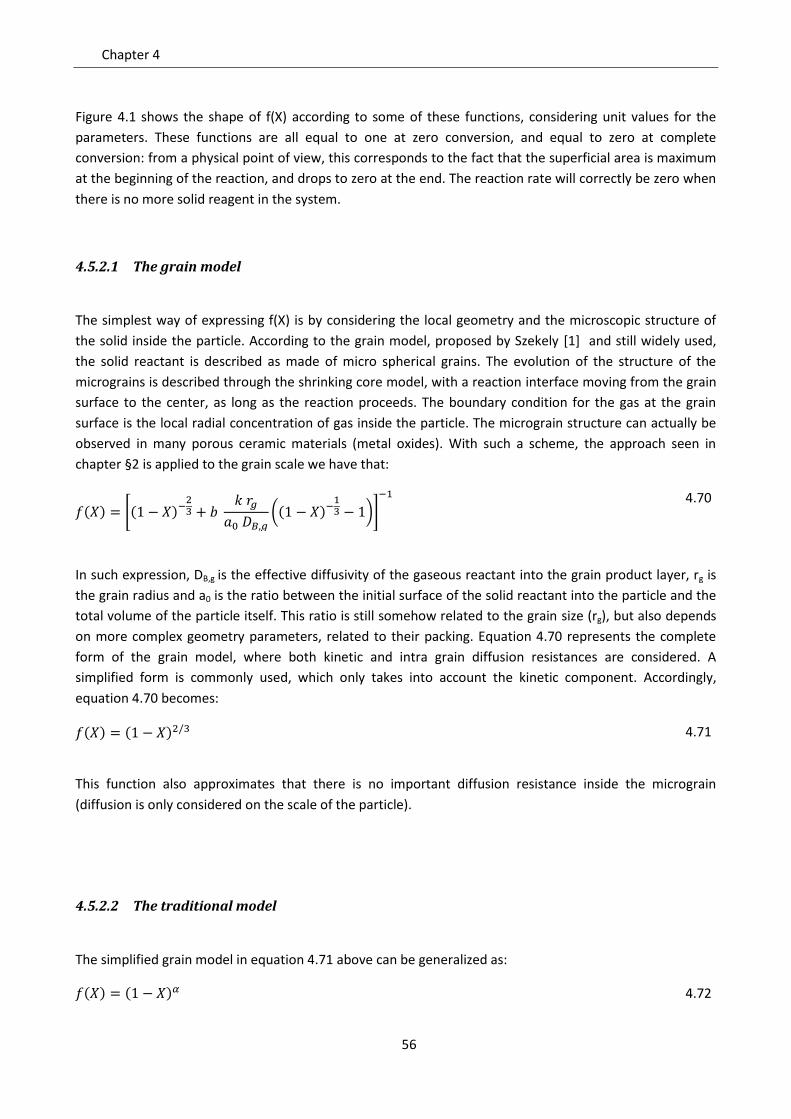
Chapter 4
56
Figure 4.1 shows the shape of f(X) according to some of these functions, considering unit values for the
parameters. These functions are all equal to one at zero conversion, and equal to zero at complete
conversion: from a physical point of view, this corresponds to the fact that the superficial area is maximum
at the beginning of the reaction, and drops to zero at the end. The reaction rate will correctly be zero when
there is no more solid reagent in the system.
4.5.2.1 The grain model
The simplest way of expressing f(X) is by considering the local geometry and the microscopic structure of
the solid inside the particle. According to the grain model, proposed by Szekely [1] and still widely used,
the solid reactant is described as made of micro spherical grains. The evolution of the structure of the
micrograins is described through the shrinking core model, with a reaction interface moving from the grain
surface to the center, as long as the reaction proceeds. The boundary condition for the gas at the grain
surface is the local radial concentration of gas inside the particle. The micrograin structure can actually be
observed in many porous ceramic materials (metal oxides). With such a scheme, the approach seen in
chapter §2 is applied to the grain scale we have that:
4.70
In such expression, DB,g is the effective diffusivity of the gaseous reactant into the grain product layer, rg is
the grain radius and a0 is the ratio between the initial surface of the solid reactant into the particle and the
total volume of the particle itself. This ratio is still somehow related to the grain size (rg), but also depends
on more complex geometry parameters, related to their packing. Equation 4.70 represents the complete
form of the grain model, where both kinetic and intra grain diffusion resistances are considered. A
simplified form is commonly used, which only takes into account the kinetic component. Accordingly,
equation 4.70 becomes:
4.71
This function also approximates that there is no important diffusion resistance inside the micrograin
(diffusion is only considered on the scale of the particle).
4.5.2.2 The traditional model
The simplified grain model in equation 4.71 above can be generalized as:
4.72
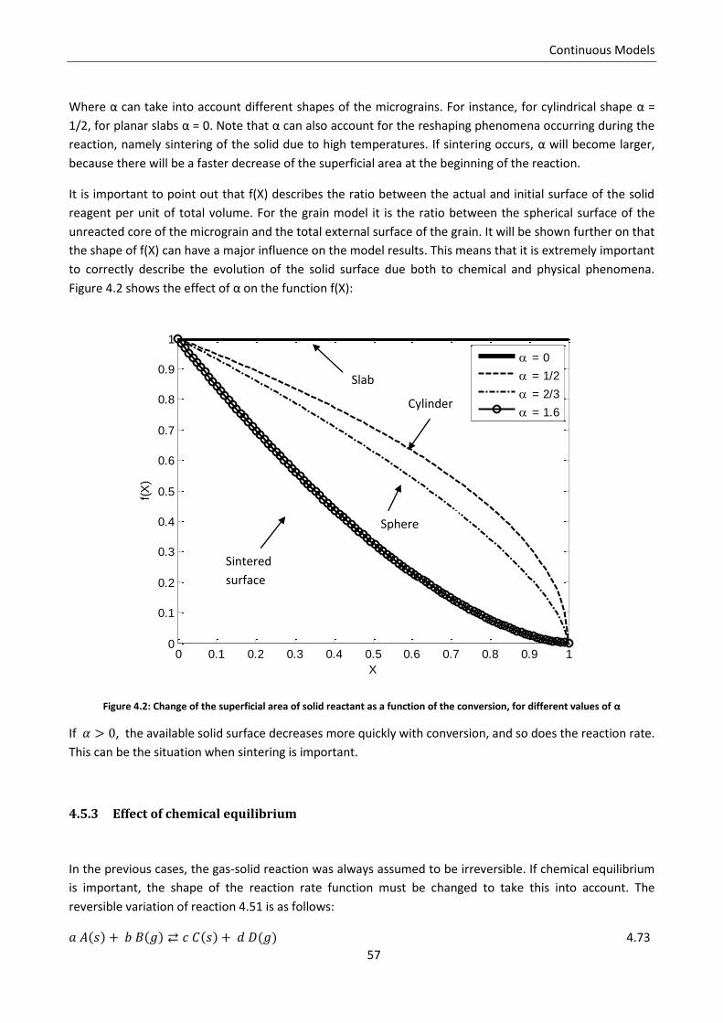
Continuous Models
57
Where α can take into account different shapes of the micrograins. For instance, for cylindrical shape α =
1/2, for planar slabs α = 0. Note that α can also account for the reshaping phenomena occurring during the
reaction, namely sintering of the solid due to high temperatures. If sintering occurs, α will become larger,
because there will be a faster decrease of the superficial area at the beginning of the reaction.
It is important to point out that f(X) describes the ratio between the actual and initial surface of the solid
reagent per unit of total volume. For the grain model it is the ratio between the spherical surface of the
unreacted core of the micrograin and the total external surface of the grain. It will be shown further on that
the shape of f(X) can have a major influence on the model results. This means that it is extremely important
to correctly describe the evolution of the solid surface due both to chemical and physical phenomena.
Figure 4.2 shows the effect of α on the function f(X):
Figure 4.2: Change of the superficial area of solid reactant as a function of the conversion, for different values of α
If , the available solid surface decreases more quickly with conversion, and so does the reaction rate.
This can be the situation when sintering is important.
4.5.3 Effect of chemical equilibrium
In the previous cases, the gas-solid reaction was always assumed to be irreversible. If chemical equilibrium
is important, the shape of the reaction rate function must be changed to take this into account. The
reversible variation of reaction 4.51 is as follows:
4.73
0 0.1 0.2 0.3 0.4 0.5 0.6 0.7 0.8 0.9 10
0.1
0.2
0.3
0.4
0.5
0.6
0.7
0.8
0.9
1
X
f(X
)
= 0
= 1/2
= 2/3
= 1.6
Sphere
Sintered
surface
Slab
Cylinder
Chapter 4
58
The form of the global reaction rate can be found by assuming that it is the sum of two reaction rates (the
direct and inverse reaction). So, applying equation 4.52, we obtain:
4.74
Now it can be remembered that the ratio between and is equal to the equilibrium constant of the
reaction, , so expression 4.74 becomes:
4.75
This expression can be used, once is calculated through thermodynamic relations.
4.6 Continuous model in terms of mass
In the previous sections, the continuous model for gas solid reactions in porous media has been described.
The material balances for both gas and solid species were expressed in terms of number of moles. The
energy balance was also developed by considering the specific enthalpies and heat capacity per unit of
moles of single species or mixture. It is also possible to formulate the same model in terms of mass, mass
fractions of the single components, mass densities, etc. The mathematical treatment of the equations is
very similar to the molar case, so we only report the final set of equations. For a spherical particle, the
model of equations 4.37-4.41 becomes:
4.76
4.77
4.78
4.79
4.80
In this formulation,
and
are the mass concentration and mass fraction of the i-th gas species,
respectively, and
are the mass concentration and mass fraction of the i-th solid species, and
Continuous Models
59
are the total mass fluxes of gas and solid, respectively, is the mass diffusive flux of the i-th gas species,
and is the molecular weight of i. The parameters inside the energy balance can be expressed as
follows:
4.81
4.82
Also in this form the total flux of gas can be calculated through equation 4.77, obtaining:
4.83
It is important to point out that this formulation of the continuous model has the same mathematical
solution as the molar set equations (4.37-4.41). Yet, the results can be different if some contributions are
neglected. This will be shown in more detail in section 6, with respect to the contribution of gas convection.
Notation
Pre exponential factor of Arrhenius law (mol,cm,s) Initial specific surface of the solid matrix (1/cm)
Molar concentration, of the i-th gas species, of the i-th solid species (mol/cm3)
Initial molar concentration, of the i-th gas species, of the i-th solid species (mol/cm
3)
Concentration of the i-th gas species outside the particle, in bulk phase (mol/cm3)
Total concentration of gas phase, of solid phase (mol/cm3)
Total concentration of combined phases (mol/cm3)
Heat capacity of the medium (J/cm3/K)
Heat capacity of the i-th gas species, of the i-th solid species (J/mol/K)
Heat capacity of the gas phase, of the solid phase (J/mol/K)
Massive heat capacity of the gas phase (J/g/K) Effective diffusivity of i into the grain
Activation energy (J/mol) Mass transfer coefficient of i (cm/s) Heat transfer coefficient (W/cm
2/K)
Enthalpy of the i-th gas species, of the i-th solid species (J/mol)
Enthalpy of the gas phase, of the solid phase (J/mol)
Chapter 4
60
Total enthalpy of combined phases (J/mol) Molar diffusive flux of i (mol/cm
2/s)
Kinetic constant, of a general reaction, of the i-th reaction step (mol, cm, s)
Thermal conductivity of the i-th gas species, of the i-th solid species (W/cm/K)
Thermal conductivity of the gas phase, of the solid phase (W/cm/K) Thermal conductivity of the medium (W/cm/K) Equilibrium constant, of a generic reaction, of the i-th reaction step Molecular weight of the i-th species (g/mol)
, Number of moles of the i-th solid species, total number of moles of solid Total mass flux of the gas phase, of the solid phase (g/cm
2/s)
Molar flux, of the i-th gas species, of the i-th solid species (mol/cm2/s)
Total molar flux of the gas phase, of the solid phase (mol/cm2/s)
Total flux of combined phases (mol/cm2/s)
Number of gas species in the system Number of reactions Number of solid species in the system Total number of species (gas + solid) P Pressure (Pa) Conductive flux (W/cm
2)
Radial coordinate (cm) Particle radius (cm) Grain radius
R Reaction rate (mol/cm3/s)
Universal gas constant (J/mol/K)
Molar source term for the i-th gas species, for the i-th solid species (mol/cm3/s )
t Time (s) Absolute temperature, local, outside the particle in bulk phase (K) Initial local temperature (K)
, Molar fraction of the i-th gas species, of the i-th solid species
Volume of solid phase, total volume (cm3)
Conversion of the A solid phase
Mass fraction of the i-th gas species, of the i-th solid species
Greek letters α Sintering exponent β Gas partial reaction order
Heat of the j-th reaction, molar based (J/mol)
Heat of the j-th reaction, mass based (J/g)
ԑ Porosity Stoichiometric coefficient of the i-th species in the j-th reaction
Stoichiometric coefficient of the i-th gas species in the j-th reaction
Stoichiometric coefficient of the i-th solid species in the j-th reaction
Intrinsic density of the i-th solid species (g/cm3)
Mass density of the i-th gas species, of the i-th solid species (g/cm3)
Mass density of the gas phase, of the solid phase (g/cm3)
Heat capacity of the medium (J/cm3/K)
Surface fraction occupied by the i-th gas phase
61
Chapter 5. Diffusion models
In the previous section, the possible forms of continuous models have been reported. In this part, the
expression of the gas diffusion fluxes in the continuous model is explicated as a function of the gas
concentration gradients, according to different degrees of detail [33, 34].
5.1 Gas diffusion and velocity
Let’s define a physical spatial domain Ω, where there is a mixture of N chemical species. In each point of
the domain a density ρ(x,y,z) and a total molar concentration c(x,y,z) can be defined. The relationship
between the two will be:
5.1
Where MW is the molecular weight of the mixture, and in general will be different in any point. Let’s
consider a subdomain ∂V in which there are Nmi molecules of the i-th species. Each molecule j of the
species i will move with a velocity . The average velocity of the species i in ∂V will be:
5.2
Each i species will move with a velocity (x,y,z). The coordinates of the center of mass of the system can
be defined as follows:
5.3
Where rj is the position of the j-th molecule, and mi is its mass. In the same way, a molar centre of mass can
be defined, whose coordinates are:
5.4
The evolution of the system in the whole volume ∂V can be summarized by describing the evolution of its
center of mass R, whose velocity will be:
5.5
Chapter 5
62
In the same way, the velocity of the molar center of mass can be defined as:
5.6
Now we recognize that:
5.7
5.8
Where yi is mass fraction of i and xi is the molar fraction of i. The equations become:
5.9
5.10
Considering the limit ∂V→0, the volume reduces to a point of Ω, with the same coordinates as R and R’
whereas the definition of vi, v and v* is still valid, and can be extended at any point of Ω. The velocity fields
vi(x,y,z), v(x,y,z) and v*(x,y,z) are thus defined.
In any point, the massive and molar total fluxes are defined as:
5.11
5.12
Massive and molar fluxes can be written for each species as well:
5.13
5.14
It’s obvious to demonstrate, by equations 5.13, 5.14, 5.9 and 5.10 that:
5.15
5.16
In practice, it’s rather useful to separate the flux of i into two components:
5.17
Diffusion models
63
5.18
Where the first term of the right hand side is the convective mass flux of i, while ji is the diffusive mass flux
of i, which is:
5.19
In terms of molar quantities:
5.20
It is easy to demonstrate that:
5.21
And analogously:
5.22
5.2 Binary and multicomponent diffusion: Fick and Stefan-Maxwell
If the system is made of only two chemical species (let’s say i and j), the massive and molar diffusive fluxes
can be expressed by the first Fick’s law:
5.23
5.24
Where Dij is the Fick binary diffusion coefficient, and depends, more or less slightly, on xi and xj. Equation
5.20 can be manipulated as follows, starting from the definition of molar diffusive fluxes:
5.25
5.26
Subtracting eq. 5.26 from eq. 5.25:
5.27
In a binary system, eq. 5.22 becomes:
5.28
Chapter 5
64
Which, substituted in equation 5.27, gives:
5.29
Now, using Fick’s law:
5.30
Which gives the explicit form of Fick’s law in terms of gradient:
5.31
Equation 5.31 is quite important, since it’s been extended for describing diffusion in multicomponent
systems where N>2. In such cases, the gradient of xi is equal to:
5.32
This equation is found to describe multicomponent diffusion with a good degree of approximation for
mixtures of gases at low pressure. At these conditions, the binary Fick coefficient gets equal to the Stefan-
Maxwell multicomponent diffusivities, Ðij, so that eq. 5.32 can be also written as:
5.33
These are the so called Stefan-Maxwell equations for ideal mixtures of gases. Multicomponent diffusivities
Ðij identify a matrix [Ð], which is symmetric (Ðij = Ðji), as well as the matrix of Fick diffusivities [ ]. The
relationship between these two kinds of coefficient is given by:
5.34
Where γi is the activity coefficient of i. In the case of ideal mixtures γi = 1, so that ij = Ðij.
Equation 5.33 is the implicit form of the Stefan-Maxwell equations. It is usually more useful to have an
expression to calculate the flux of i as a function of the gradients of the molar fractions of the components.
This can be obtained for a multicomponent system, by manipulating equation 5.33 as follows:
Using equations 5.25 and 5.26:
5.35
Diffusion models
65
Equation 5.35 says that the gradient of i depends on N molar fluxes, as many as the number of components
of the system. Actually, it depends on N-1 fluxes, since the N-th flux can be obtained, according to equation
5.22, as:
5.36
In equation 5.35 we can thus extract the N-th member of the last sum, and use equation 5.36 to eliminate
the N-th molar flux. We obtain:
5.37
5.38
We can now extract the i-th component from both sums of the right hand side of equation 5.38:
5.39
Simplifying the term with :
5.40
And, in a more compact way:
5.41
Where δij is the delta of Kronecker, which is equal to 1 if i = j and is equal to zero otherwise.
We can define an (N-1xN-1) matrix [B], where the component Bij is given by:
5.42
So that equation 5.41 becomes:
Chapter 5
66
5.43
Or, in a matrix form:
5.44
Where is the (N-1x1) column vector of the gradients of the components, and is the (N-1x1)
column vector of the molar fluxes. N-1 fluxes can be calculated by resolving the linear system expressed by
eq. 5.44, so that:
5.45
We define [D] as the inverse matrix of B, thus obtaining:
5.46
Or, in a more explicit form:
5.47
This is the so called generalized Fick’s law, and is actually a manipulated version of the Stefan-Maxwell
equations. Equation 5.46, together with equation 5.36, gives the total of N diffusive fluxes necessary to
describe the system. Note that eq. 5.47 is not fully explicit, as it requires that the matrix B, depending on
the compositions xi, is inverted.
5.3 Other forms of the Stefan-Maxwell equations
There is a number of ways to express equation 5.33 rather than equation 5.47. In particular, it can be useful
to calculate the mass fluxes instead of the molar ones. Here we consider two common expression of the
generalized Fick’s equation.
5.48
5.49
First of all, we can obtain the relationship between the mass and molar fluxes as follows. The difference
between the velocity of the center of mass and the velocity of molar center of mass is:
5.50
Diffusion models
67
Where expression 5.9 is used to express v. We can multiply v* by the sum of yi, which we know to be equal
to one, so that:
5.51
Now we can use equation 5.51 into the definition of ji, and we obtain:
5.52
And using the definition of J*i:
5.53
Extracting the N-th molar flux from the sum and applying the condition on the sum of the fluxes we obtain:
5.54
Now, extracting the i-th element from the sum:
5.55
Or, in a more contract form:
5.56
So we obtain:
5.57
Chapter 5
68
5.58
As well as:
5.59
5.60
Or, in matrix form:
5.61
5.62
Combining equation 5.62 and 5.46 we obtain the following expression:
5.63
So we obtained the transformation:
5.64
5.65
Which is the matrix form of equation 5.48.
To compute the matrix [D°], we first calculate the transformation from to , knowing that:
5.66
Using the derivation rules:
5.67
Where the molecular weight of the mixture, MW, is defined as:
Diffusion models
69
5.68
We again extract the N-th element from the sum in equation:
5.69
Then we use the relation:
5.70
So that we get:
5.71
Then, extracting the i-th element:
5.72
5.73
Now we define the transformation matrix [Bxy] whose elements are given by:
5.74
It is also possible to prove that BF is the inverse of Bxy.
So the relationship between molar and mass gradients is:
5.75
5.76
Finally we can combine equations 5.61, 5.46 and 5.76, so we obtain:
5.77
Chapter 5
70
That give us the formulation of the diffusivity matrix [D°]:
5.78
5.79
This is the generalized Fick equation in terms of mass fluxes as a function of the gradients of the mass
fractions.
5.3.1 From multicomponent to binary form
We can easily demonstrate that, if N = 2, we obtain the binary Fick law from the equations we just derived.
The matrix [B], if N = 2 has only one component which is:
5.80
And so:
5.81
5.82
The matrix [BF], has a single component as well, which is:
5.83
While the matrix [Bxy] is:
5.84
So the matrix [D°] will be:
5.85
5.86
Diffusion models
71
Finally, if one of the two species is very diluted with respect to the other one,
5.87
Because γ1 1 if x1 0 or x1 1.
Thus, we obtained the same forms as equations 5.23 and 5.24.
5.3.2 Alternative (direct) way to derive SM-equation in term of massive fluxes
It is possible to directly derive the matrix [D*] combining equations 5.33 and 5.20:
5.88
With the same logical rearrangements we obtain:
5.89
5.90
It’s immediate to recognize that [D*] = [B*]-1
5.4 Contribution of Knudsen diffusion
If the diffusion regime can be influenced by Knudsen diffusion, equation 5.42 can be corrected as reported
in the literature [9], as follows:
5.91
Where DiK is the Knudsen diffusion coefficient of i, which can be expressed by:
5.92
Chapter 5
72
Where K0 is the Knudsen parameter, depending on the conformation of the solid medium. This extension
adds a new term in the diagonal of the matrix [B], whose component will be:
5.93
Note that if DiK approaches to infinite, Knudsen diffusion is no longer important, and equation 5.93 returns
to be in the form of equation 5.42.
5.5 Generalized Stefan-Maxwell for multiple driving forces and non ideal
solutions
Thus far, we considered concentration differences as the only source of a diffusive flux, and for ideal
mixtures. In general, diffusion can be generated by other non homogeneous properties in the system, such
as:
a) Temperature gradients b) Pressure gradients c) External forces
In order to take into account all of these, the generalized Fick equation expressed by 5.47 has been
extended into equation 5.94:
5.94
5.95
Where ai is the activity of i, φi is the volumetric fraction of i, P is the pressure, T is the temperature, and gi is
the external force field applied to i. It may include, for example, gravity force, electric fields caused by ionic
forces, permeability differences due to the presence of selective membranes. For more details about these
ones, we remand to the literature [33]. DTi is the thermal diffusion coefficient of i, while D*ij is still
calculated by the inversion of the matrix in eq. 5.90. It can be demonstrated that the sum of the driving
forces of all the components must always be equal to zero:
5.96
Note that the contribution of the concentration gradient in this formulation is expressed by the first term of
the right hand side of equation 5.95. For non ideal systems, Dij and Ðij are not interchangeable, and the
Diffusion models
73
activity of i is different from its molar fraction. The comparison between the generalized form of the Stefan
Maxwell equations and the Fick equation 5.23 gives the relationship between the two coefficients, already
exposed in 5.34.
5.6 Simplified diffusion models: Mixture averaged model
The Stefan-Maxwell multicomponent diffusion is the most rigorous approach to describe the molar or
massive diffusive fluxes in a system with more than two chemical species. It can be nevertheless quite
annoying to use, because of its intrinsic implicit form, that requires the inversion of a matrix (B), whose
components are different in any point of the system at any numerical iteration. This can result in a more
expensive computational cost in the numerical solution of the material balances, particularly if N is very
large. A simplified approach can be used, in order to have a fully explicit equation to calculate the diffusive
fluxes, maintaining an approximate dependence on the composition of the system.
One widely used approach is to calculate a global diffusion coefficient, so that the diffusive flux of i is
expressed in the form of the binary Fick law. For the molar flux:
5.97
Where Dim is the diffusion coefficient of i in the mixture. This diffusivity can be exactly calculated,
comparing equations 5.97 and 5.35:
5.98
So we obtain:
5.99
Now using equations 5.16 and 5.18 into equation 5.99 we can express Dim as a function of the global molar
fluxes:
5.100
Finally:
5.101
Chapter 5
74
Note that the combination of equations 5.101 and 5.97 is still another form of equation 5.33. If the molar
flux of i is very large compared to the fluxes of the other species, then Ni = N, and Nj = 0, for j different from
i. The diffusivity becomes:
5.102
Dim still depends on the composition of the system (x) and on the multicomponent diffusivities, but not on
the molar fluxes, so it’s fully explicit.
5.6.1 Derivation of mass fluxes
Another common form of the mixture averaged model is through equation 5.103:
5.103
Starting from equations 5.35 and 5.19:
5.104
5.105
In terms of global massive fluxes:
5.106
Again, if ni is nearly equal to n:
5.107
Equation 5.103 can be also expressed in terms of massive fraction as (Comsol MPh form):
5.108
Diffusion models
75
5.7 Effective diffusion coefficients
One final issue related to the correct description of diffusion phenomena regards effective diffusion
coefficients. In the previous sections, diffusion models were described assuming that the gas species can
diffuse in an open domain. In porous media, gas has to go through the pores and spaces present inside a
solid matrix. The conventional diffusion models could be applied only if the pores domain was simulated,
which implies the exact description of the local multiphase geometry inside the particle. This is almost
never feasible, even if theoretical studies are made in this sense [35], [36]. A common approach implies the
description of the gas-solid matrix as a continuum, with the properties of gas and solid species that can be
calculated in any point. In order to describe diffusion, the same mathematical models presented before are
used, but with effective diffusion coefficients scaled by local porosity and tortuosity . For instance, the
diffusion coefficients of the generalized Fick’s law for the molar diffusion fluxes (equation 5.47) become:
5.109
The same approximation can be applied to the binary Fick’s law and Mixture averaged models, both in
molar and mass form. Porosity and tortuosity are properties of the solid matrix. Porosity can be calculated
according to mass balances inside the particle, whereas tortuosity is much more difficult to quantify, and
usually is considered as a parameter of the problem.
Notation
Activity of i Components of the inverse of Stefan-Maxwell diffusion matrix (s/cm
2)
,
Matrices of transformation from molar diffusion fluxes to mass diffusion fluxes
Matrix of transformation from the gradients of y to the gradients of x
Total gas concentration (mol/cm3)
Binary Fick diffusion coefficient of i in j (cm2/s)
Multicomponent diffusion coefficient of i in j (cm2/s)
Components of the Stefan-Maxwell diffusion matrix (cm2/s)
Effective Stefan-Maxwell diffusion coefficient (cm2/s)
Multicomponent diffusivities to express as a function of the gradients of x (cm
2/s)
Multicomponent diffusivities to express as a function of the gradients of y (cm
2/s)
Knudsen diffusion coefficient of i (cm
2/s)
Thermal diffusion coefficient if i (cm
2/s)
Diffusion coefficients of i in the gas mixture, for the molar and mass fluxes (cm
2/s)
External force field applied to i (J/g) Mass diffusive flux of i (g/cm
2/s)
Molar diffusive flux of i (mol/cm
2/s)
Knudsen number Mass of the i-th molecule or species (g)
Chapter 5
76
Molecular weight of gas phase (g/mol) Molecular weight of the i-th species (g/mol) Total mass flux of the gas phase, of the gas i-th species (g/cm
2/s)
Number of gas species in the system , Total molar flux of the gas phase, of the i-th gas species (mol/cm
2/s)
Number of molecules of the i-th species Total number of gas molecules P Pressure (Pa) Position of the center of mass (cm) Position of the molar center of mass (cm) Universal gas constant (J/mol/K)
Position of the j-th molecule (cm)
Absolute temperature (K) Velocity of the i-th species (cm/s) Velocity of the j-th molecule of the i-th species (cm/s)
Velocity of the gas center of mass (cm/s) Velocity of the gas molar center of mass (cm/s) Molar fraction of the i-th gas species Mass fraction of the i-th gas species Greek letters Activity coefficient of i ԑ Porosity Volume fraction of i Gas density (g/cm
3)
Tortuosity
77
Chapter 6. Role of diffusion and convection in particle models
In the previous section, different approaches to describe gas diffusion were discussed. The multicomponent
Stefan Maxwell model is the most correct when dealing with gas mixtures with more than two species
involved. From a mathematical point of view, it is also the most difficult to implement, for two main
reasons: first because the diffusive flux of one species depends on the concentration gradients of all the
species in the system, so this model introduces other terms of coupling between the equations to solve;
second but not less important, it introduces non linearities, in the calculation of the diffusion matrix. Even if
the diffusion matrix usually depends weakly on the gas composition, a more complex numerical treatment
is necessary to solve the problem. In many cases it can be convenient to use a simpler Fick’s law, with
constant diffusion coefficients, possibly scaled with the local porosity, or expressed as a function of the gas
composition, like in the mixture averaged model.
All the simplifications may lead to inaccuracies in the description of gas diffusion, and in the model results.
Several factors can affect these inaccuracies:
a) The importance of diffusion with respect to the other resistances: if diffusion is fast compared
to chemical reaction (chemical regime) it is more likely that the choice of the diffusion model
makes little or no difference in the estimated conversion results. On the contrary, if diffusion is
the rate determining step it can be worth to be more accurate on the description of the gas
transport inside the particle. The controlling regime can depend on many factors: the particle
size may also play an important role.
b) The number of species in the gas mixture. It can be demonstrated that all the multicomponent
diffusion models become identical to the binary Fick’s law if only two species are present in the
system. The more species, the more it is likely that a multicomponent model is necessary.
c) The values of the binary diffusion coefficients: it can be proved that the Stefan Maxwell model
becomes identical to the binary Fick’s law if all the binary diffusion coefficients are the same.
On the contrary, major differences can arise if they are very different from each others. This
happens for example if there are molecules with different volumes: a typical example of a
critical mixture is when hydrogen is present, because of its higher diffusivity if compared to
those of other gases.
d) The degree of dilution of the gas species. If the fraction of one species is very high if compared
to the others, the multicomponent model becomes similar to the Fick’s law, where the diffusion
coefficients used are the diffusivities of the diluted species into the diluents.
6.1 Mathematical proof of model simplifications
In the following we provide mathematical proofs of the simplifications of SM to Fick’s law for the four cases
listed above. Let us consider the inverse of the multicomponent diffusion matrix as expressed in equation
5.42, and here reported again:
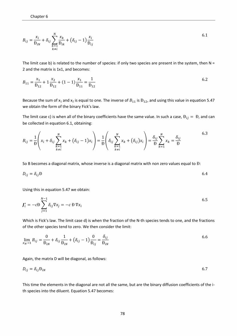
Chapter 6
78
6.1
The limit case b) is related to the number of species: if only two species are present in the system, then N =
2 and the matrix is 1x1, and becomes:
6.2
Because the sum of x1 and x2 is equal to one. The inverse of is , and using this value in equation 5.47
we obtain the form of the binary Fick’s law.
The limit case c) is when all of the binary coefficients have the same value. In such a case, , and can
be collected in equation 6.1, obtaining:
6.3
So B becomes a diagonal matrix, whose inverse is a diagonal matrix with non zero values equal to :
6.4
Using this in equation 5.47 we obtain:
6.5
Which is Fick’s law. The limit case d) is when the fraction of the N-th species tends to one, and the fractions
of the other species tend to zero. We then consider the limit:
6.6
Again, the matrix D will be diagonal, as follows:
6.7
This time the elements in the diagonal are not all the same, but are the binary diffusion coefficients of the i-
th species into the diluent. Equation 5.47 becomes:
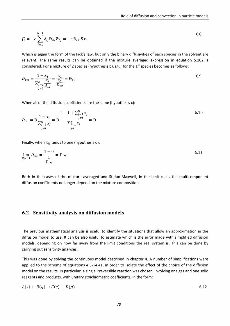
Role of diffusion and convection in particle models
79
6.8
Which is again the form of the Fick’s law, but only the binary diffusivities of each species in the solvent are
relevant. The same results can be obtained if the mixture averaged expression in equation 5.102 is
considered. For a mixture of 2 species (hypothesis b), for the 1st species becomes as follows:
6.9
When all of the diffusion coefficients are the same (hypothesis c):
6.10
Finally, when tends to one (hypothesis d):
6.11
Both in the cases of the mixture averaged and Stefan-Maxwell, in the limit cases the multicomponent
diffusion coefficients no longer depend on the mixture composition.
6.2 Sensitivity analysis on diffusion models
The previous mathematical analysis is useful to identify the situations that allow an approximation in the
diffusion model to use. It can be also useful to estimate which is the error made with simplified diffusion
models, depending on how far away from the limit conditions the real system is. This can be done by
carrying out sensitivity analyses.
This was done by solving the continuous model described in chapter 4. A number of simplifications were
applied to the scheme of equations 4.37-4.41, in order to isolate the effect of the choice of the diffusion
model on the results. In particular, a single irreversible reaction was chosen, involving one gas and one solid
reagents and products, with unitary stoichiometric coefficients, in the form:
6.12
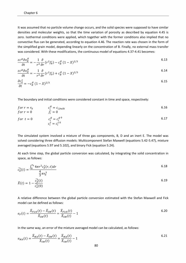
Chapter 6
80
It was assumed that no particle volume change occurs, and the solid species were supposed to have similar
densities and molecular weights, so that the time variation of porosity as described by equation 4.45 is
zero. Isothermal conditions were applied, which together with the former conditions also implied that no
convective flux can be generated, according to equation 4.46. The reaction rate was chosen in the form of
the simplified grain model, depending linearly on the concentration of B. Finally, no external mass transfer
was considered. With these modifications, the continuous model of equations 4.37-4.41 becomes:
6.13
6.14
6.15
The boundary and initial conditions were considered constant in time and space, respectively:
6.16
6.17
The simulated system involved a mixture of three gas components, B, D and an inert E. The model was
solved considering three diffusion models: Multicomponent Stefan Maxwell (equations 5.42-5.47), mixture
averaged (equations 5.97 and 5.102), and binary Fick (equation 5.24).
At each time step, the global particle conversion was calculated, by integrating the solid concentration in
space, as follows:
6.18
6.19
A relative difference between the global particle conversion estimated with the Stefan Maxwell and Fick
model can be defined as follows:
6.20
In the same way, an error of the mixture averaged model can be calculated, as follows:
6.21
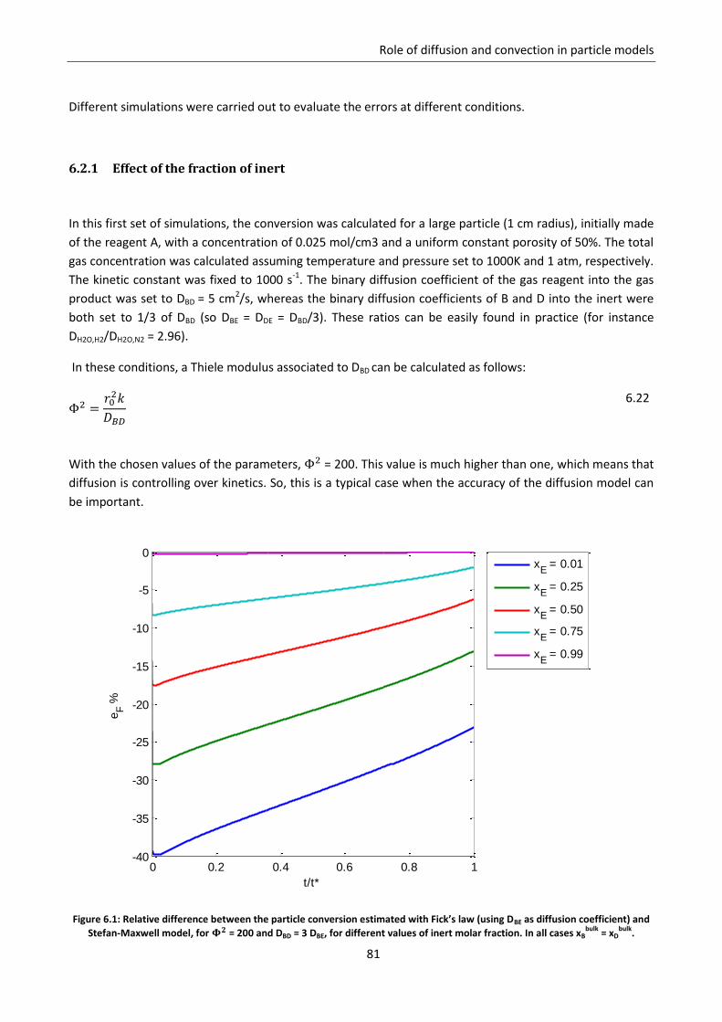
Role of diffusion and convection in particle models
81
Different simulations were carried out to evaluate the errors at different conditions.
6.2.1 Effect of the fraction of inert
In this first set of simulations, the conversion was calculated for a large particle (1 cm radius), initially made
of the reagent A, with a concentration of 0.025 mol/cm3 and a uniform constant porosity of 50%. The total
gas concentration was calculated assuming temperature and pressure set to 1000K and 1 atm, respectively.
The kinetic constant was fixed to 1000 s-1. The binary diffusion coefficient of the gas reagent into the gas
product was set to DBD = 5 cm2/s, whereas the binary diffusion coefficients of B and D into the inert were
both set to 1/3 of DBD (so DBE = DDE = DBD/3). These ratios can be easily found in practice (for instance
DH2O,H2/DH2O,N2 = 2.96).
In these conditions, a Thiele modulus associated to DBD can be calculated as follows:
6.22
With the chosen values of the parameters, = 200. This value is much higher than one, which means that
diffusion is controlling over kinetics. So, this is a typical case when the accuracy of the diffusion model can
be important.
Figure 6.1: Relative difference between the particle conversion estimated with Fick’s law (using DBE as diffusion coefficient) and
Stefan-Maxwell model, for = 200 and DBD = 3 DBE, for different values of inert molar fraction. In all cases xBbulk
= xDbulk
.
0 0.2 0.4 0.6 0.8 1-40
-35
-30
-25
-20
-15
-10
-5
0
t/t*
eF %
x
E = 0.01
xE = 0.25
xE = 0.50
xE = 0.75
xE = 0.99
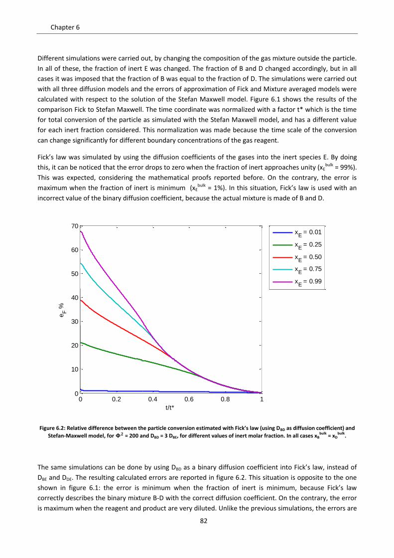
Chapter 6
82
Different simulations were carried out, by changing the composition of the gas mixture outside the particle.
In all of these, the fraction of inert E was changed. The fraction of B and D changed accordingly, but in all
cases it was imposed that the fraction of B was equal to the fraction of D. The simulations were carried out
with all three diffusion models and the errors of approximation of Fick and Mixture averaged models were
calculated with respect to the solution of the Stefan Maxwell model. Figure 6.1 shows the results of the
comparison Fick to Stefan Maxwell. The time coordinate was normalized with a factor t* which is the time
for total conversion of the particle as simulated with the Stefan Maxwell model, and has a different value
for each inert fraction considered. This normalization was made because the time scale of the conversion
can change significantly for different boundary concentrations of the gas reagent.
Fick’s law was simulated by using the diffusion coefficients of the gases into the inert species E. By doing
this, it can be noticed that the error drops to zero when the fraction of inert approaches unity (xEbulk = 99%).
This was expected, considering the mathematical proofs reported before. On the contrary, the error is
maximum when the fraction of inert is minimum (xEbulk = 1%). In this situation, Fick’s law is used with an
incorrect value of the binary diffusion coefficient, because the actual mixture is made of B and D.
Figure 6.2: Relative difference between the particle conversion estimated with Fick’s law (using DBD as diffusion coefficient) and
Stefan-Maxwell model, for = 200 and DBD = 3 DBE, for different values of inert molar fraction. In all cases xBbulk
= xDbulk
.
The same simulations can be done by using DBD as a binary diffusion coefficient into Fick’s law, instead of
DBE and DDE. The resulting calculated errors are reported in figure 6.2. This situation is opposite to the one
shown in figure 6.1: the error is minimum when the fraction of inert is minimum, because Fick’s law
correctly describes the binary mixture B-D with the correct diffusion coefficient. On the contrary, the error
is maximum when the reagent and product are very diluted. Unlike the previous simulations, the errors are
0 0.2 0.4 0.6 0.8 10
10
20
30
40
50
60
70
t/t*
eF %
x
E = 0.01
xE = 0.25
xE = 0.50
xE = 0.75
xE = 0.99
Role of diffusion and convection in particle models
83
positive in this case, because DBD is higher than DBE, and so the simplified model doesn’t account for a more
difficult diffusion into the inert, which results in an overestimation of the particle conversion. The error
profiles seem to converge to a single line dropping to zero with time. This is just due to the fact that there is
a time t < t* when Fick’s law predicts full conversion of the particle, whereas for the Stefan Maxwell model
the reaction is still going on. From that time on, the predicted conversion with Fick’s law is always one,
while the predicted conversion with Stefan Maxwell approaches one. As a result, the difference between
the two models drops to zero. If the errors are negative this doesn’t happen, because at t = t* the SM
model predicts full conversion whereas according to the simplified model the reaction is still going on.
It can be noticed that the errors made with Fick’s law can be very consistent for the considered cases (more
than 50%). In general, the approximation using the diffusion coefficients related to the inert seems more
accurate than the one using the binary coefficient of B in D, getting far away from the conditions of
applicability of Fick’s law.
Figure 6.3: Relative difference between the particle conversion estimated with Mixture Averaged model and Stefan-Maxwell
model, for = 200 and DBD = 3 DBE, for different values of inert molar fraction. In all cases xBbulk
= xDbulk
.
Figure 6.3 shows the comparison of the results obtained with Mixture averaged and Stefan Maxwell model.
In this test, the estimated diffusion coefficients in the mixture ( ) were calculated from the same set of
binary diffusion coefficients as before. As expected, the Mixture averaged is much more accurate than
Fick’s law, because somehow it accounts for the effect of the local gas composition, even if not in the most
rigorous way. The calculated errors are quite lower in this case. The errors drop to zero on both the limit
cases (extreme dilution or no dilution of B and D). This is also consistent with what was proved in equations
6.2, 6.6 , 6.9 and 6.11. In this case the absolute error is maximum at intermediate conditions (50% of inert
0 0.2 0.4 0.6 0.8 1-4
-3.5
-3
-2.5
-2
-1.5
-1
-0.5
0
0.5
1
t/t*
eM
A %
x
E = 0.01
xE = 0.25
xE = 0.50
xE = 0.75
xE = 0.99
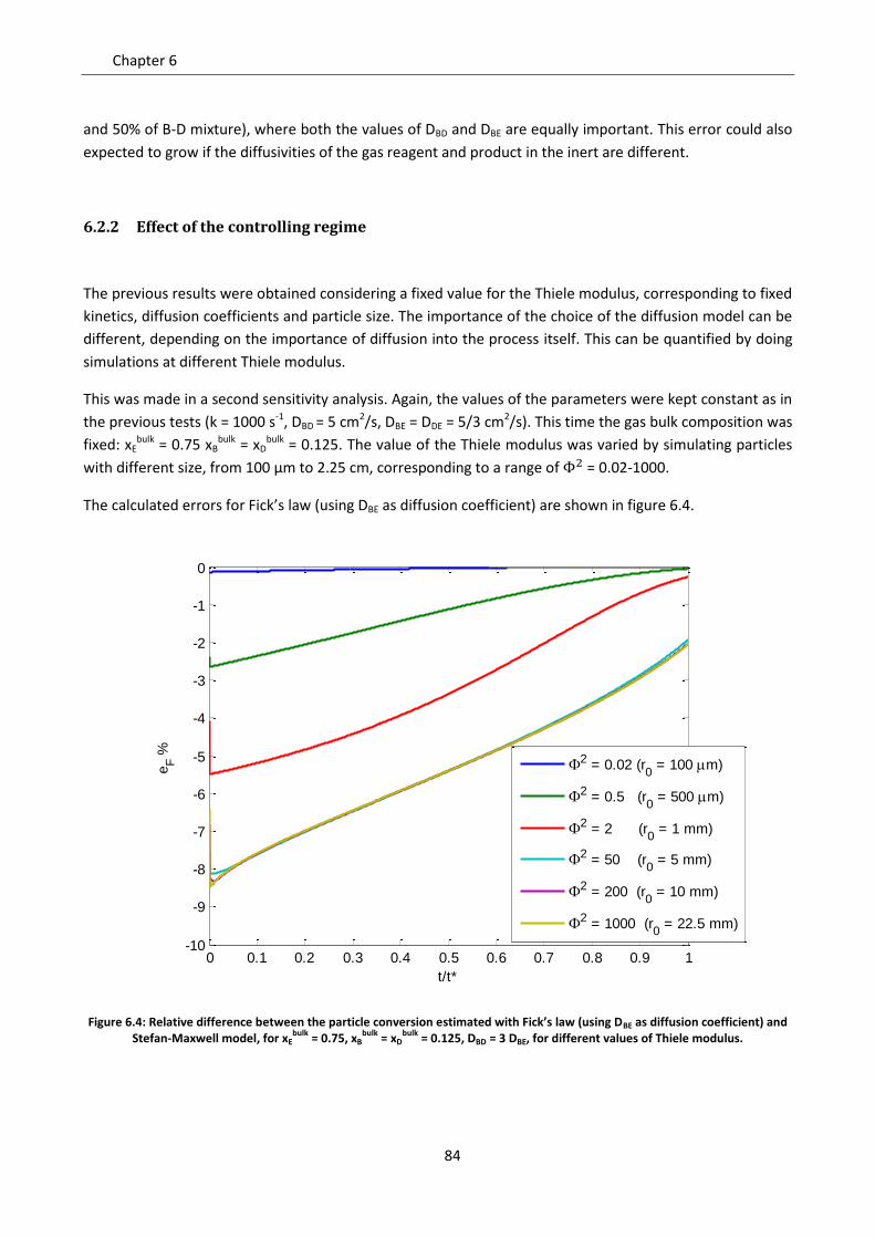
Chapter 6
84
and 50% of B-D mixture), where both the values of DBD and DBE are equally important. This error could also
expected to grow if the diffusivities of the gas reagent and product in the inert are different.
6.2.2 Effect of the controlling regime
The previous results were obtained considering a fixed value for the Thiele modulus, corresponding to fixed
kinetics, diffusion coefficients and particle size. The importance of the choice of the diffusion model can be
different, depending on the importance of diffusion into the process itself. This can be quantified by doing
simulations at different Thiele modulus.
This was made in a second sensitivity analysis. Again, the values of the parameters were kept constant as in
the previous tests (k = 1000 s-1, DBD = 5 cm2/s, DBE = DDE = 5/3 cm2/s). This time the gas bulk composition was
fixed: xEbulk = 0.75 xB
bulk = xDbulk = 0.125. The value of the Thiele modulus was varied by simulating particles
with different size, from 100 µm to 2.25 cm, corresponding to a range of = 0.02-1000.
The calculated errors for Fick’s law (using DBE as diffusion coefficient) are shown in figure 6.4.
Figure 6.4: Relative difference between the particle conversion estimated with Fick’s law (using DBE as diffusion coefficient) and Stefan-Maxwell model, for xE
bulk = 0.75, xB
bulk = xD
bulk = 0.125, DBD = 3 DBE, for different values of Thiele modulus.
0 0.1 0.2 0.3 0.4 0.5 0.6 0.7 0.8 0.9 1-10
-9
-8
-7
-6
-5
-4
-3
-2
-1
0
t/t*
eF %
2 = 0.02 (r0 = 100 m)
2 = 0.5 (r0 = 500 m)
2 = 2 (r0 = 1 mm)
2 = 50 (r0 = 5 mm)
2 = 200 (r0 = 10 mm)
2 = 1000 (r0 = 22.5 mm)
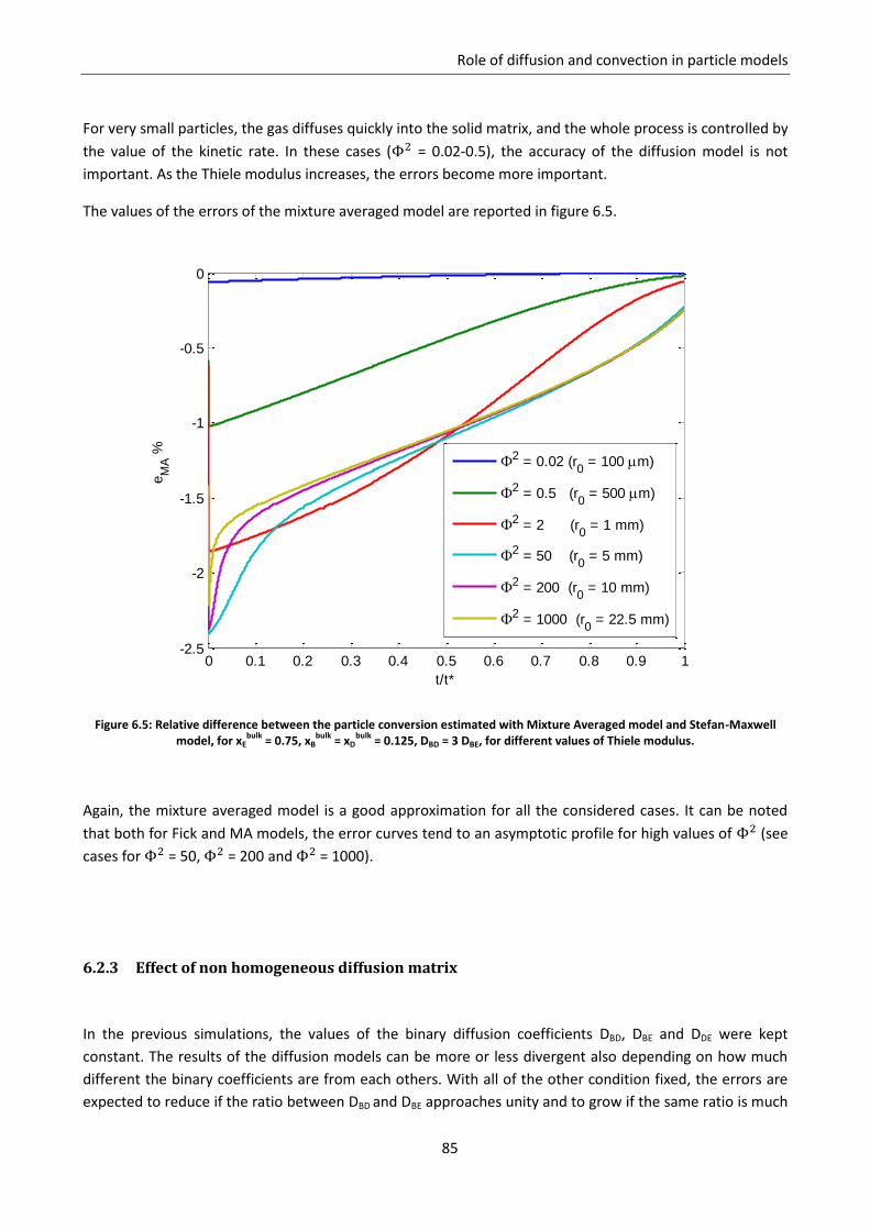
Role of diffusion and convection in particle models
85
For very small particles, the gas diffuses quickly into the solid matrix, and the whole process is controlled by
the value of the kinetic rate. In these cases ( = 0.02-0.5), the accuracy of the diffusion model is not
important. As the Thiele modulus increases, the errors become more important.
The values of the errors of the mixture averaged model are reported in figure 6.5.
Figure 6.5: Relative difference between the particle conversion estimated with Mixture Averaged model and Stefan-Maxwell model, for xE
bulk = 0.75, xB
bulk = xD
bulk = 0.125, DBD = 3 DBE, for different values of Thiele modulus.
Again, the mixture averaged model is a good approximation for all the considered cases. It can be noted
that both for Fick and MA models, the error curves tend to an asymptotic profile for high values of (see
cases for = 50, = 200 and = 1000).
6.2.3 Effect of non homogeneous diffusion matrix
In the previous simulations, the values of the binary diffusion coefficients DBD, DBE and DDE were kept
constant. The results of the diffusion models can be more or less divergent also depending on how much
different the binary coefficients are from each others. With all of the other condition fixed, the errors are
expected to reduce if the ratio between DBD and DBE approaches unity and to grow if the same ratio is much
0 0.1 0.2 0.3 0.4 0.5 0.6 0.7 0.8 0.9 1-2.5
-2
-1.5
-1
-0.5
0
t/t*
eM
A %
2 = 0.02 (r0 = 100 m)
2 = 0.5 (r0 = 500 m)
2 = 2 (r0 = 1 mm)
2 = 50 (r0 = 5 mm)
2 = 200 (r0 = 10 mm)
2 = 1000 (r0 = 22.5 mm)
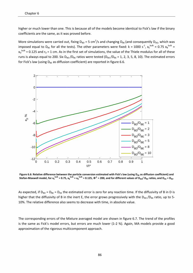
Chapter 6
86
higher or much lower than one. This is because all of the models become identical to Fick’s law if the binary
coefficients are the same, as it was proved before.
More simulations were carried out, fixing DBD = 5 cm2/s and changing DBE (and consequently DDE, which was
imposed equal to DBE for all the tests). The other parameters were fixed: k = 1000 s-1, xEbulk = 0.75 xB
bulk =
xDbulk = 0.125 and r0 = 1 cm. As in the first set of simulations, the value of the Thiele modulus for all of these
runs is always equal to 200. Six DBD /DBE ratios were tested (DBD /DBE = 1, 2, 3, 5, 8, 10). The estimated errors
for Fick’s law (using DBE as diffusion coefficient) are reported in figure 6.6.
Figure 6.6: Relative difference between the particle conversion estimated with Fick’s law (using DBE as diffusion coefficient) and
Stefan-Maxwell model, for xEbulk
= 0.75, xBbulk
= xDbulk
= 0.125, = 200, and for different values of DBD/ DBE ratios, and DDE = DBE.
As expected, if DBD = DBE = DDE the estimated error is zero for any reaction time. If the diffusivity of B in D is
higher that the diffusivity of B in the inert E, the error grows progressively with the DBD /DBE ratio, up to 5-
10%. The relative difference also seems to decrease with time, in absolute value.
The corresponding errors of the Mixture averaged model are shown in figure 6.7. The trend of the profiles
is the same as Fick’s model errors, but errors are much lower (1-2 %). Again, MA models provide a good
approximation of the rigorous multicomponent approach.
0 0.1 0.2 0.3 0.4 0.5 0.6 0.7 0.8 0.9 1-12
-10
-8
-6
-4
-2
0
2
t/t*
eF %
DBD
/DBE
= 1
DBD
/DBE
= 2
DBD
/DBE
= 3
DBD
/DBE
= 5
DBD
/DBE
= 8
DBD
/DBE
= 10
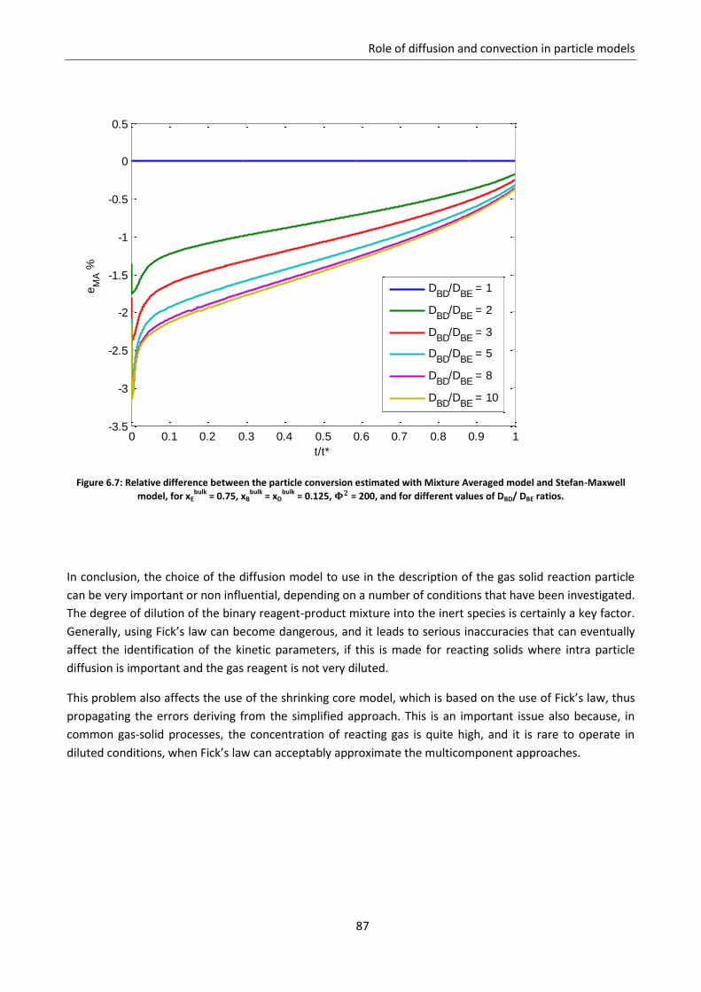
Role of diffusion and convection in particle models
87
Figure 6.7: Relative difference between the particle conversion estimated with Mixture Averaged model and Stefan-Maxwell
model, for xEbulk
= 0.75, xBbulk
= xDbulk
= 0.125, = 200, and for different values of DBD/ DBE ratios.
In conclusion, the choice of the diffusion model to use in the description of the gas solid reaction particle
can be very important or non influential, depending on a number of conditions that have been investigated.
The degree of dilution of the binary reagent-product mixture into the inert species is certainly a key factor.
Generally, using Fick’s law can become dangerous, and it leads to serious inaccuracies that can eventually
affect the identification of the kinetic parameters, if this is made for reacting solids where intra particle
diffusion is important and the gas reagent is not very diluted.
This problem also affects the use of the shrinking core model, which is based on the use of Fick’s law, thus
propagating the errors deriving from the simplified approach. This is an important issue also because, in
common gas-solid processes, the concentration of reacting gas is quite high, and it is rare to operate in
diluted conditions, when Fick’s law can acceptably approximate the multicomponent approaches.
0 0.1 0.2 0.3 0.4 0.5 0.6 0.7 0.8 0.9 1-3.5
-3
-2.5
-2
-1.5
-1
-0.5
0
0.5
t/t*
eM
A %
DBD
/DBE
= 1
DBD
/DBE
= 2
DBD
/DBE
= 3
DBD
/DBE
= 5
DBD
/DBE
= 8
DBD
/DBE
= 10
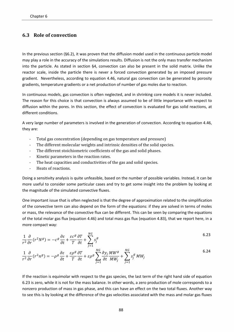
Chapter 6
88
6.3 Role of convection
In the previous section (§6.2), it was proven that the diffusion model used in the continuous particle model
may play a role in the accuracy of the simulations results. Diffusion is not the only mass transfer mechanism
into the particle. As stated in section §4, convection can also be present in the solid matrix. Unlike the
reactor scale, inside the particle there is never a forced convection generated by an imposed pressure
gradient. Nevertheless, according to equation 4.46, natural gas convection can be generated by porosity
gradients, temperature gradients or a net production of number of gas moles due to reaction.
In continuous models, gas convection is often neglected, and in shrinking core models it is never included.
The reason for this choice is that convection is always assumed to be of little importance with respect to
diffusion within the pores. In this section, the effect of convection is evaluated for gas solid reactions, at
different conditions.
A very large number of parameters is involved in the generation of convection. According to equation 4.46,
they are:
- Total gas concentration (depending on gas temperature and pressure)
- The different molecular weights and intrinsic densities of the solid species.
- The different stoichiometric coefficients of the gas and solid phases.
- Kinetic parameters in the reaction rates.
- The heat capacities and conductivities of the gas and solid species.
- Heats of reactions.
Doing a sensitivity analysis is quite unfeasible, based on the number of possible variables. Instead, it can be
more useful to consider some particular cases and try to get some insight into the problem by looking at
the magnitude of the simulated convective fluxes.
One important issue that is often neglected is that the degree of approximation related to the simplification
of the convective term can also depend on the form of the equations: if they are solved in terms of moles
or mass, the relevance of the convective flux can be different. This can be seen by comparing the equations
of the total molar gas flux (equation 4.46) and total mass gas flux (equation 4.83), that we report here, in a
more compact way:
6.23
6.24
If the reaction is equimolar with respect to the gas species, the last term of the right hand side of equation
6.23 is zero, while it is not for the mass balance. In other words, a zero production of mole corresponds to a
nonzero production of mass in gas phase, and this can have an effect on the two total fluxes. Another way
to see this is by looking at the difference of the gas velocities associated with the mass and molar gas fluxes
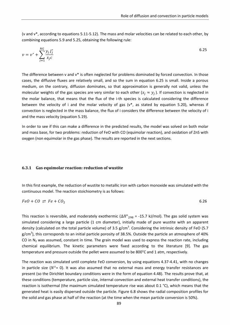
Role of diffusion and convection in particle models
89
(v and v*, according to equations 5.11-5.12). The mass and molar velocities can be related to each other, by
combining equations 5.9 and 5.25, obtaining the following rule:
6.25
The difference between v and v* is often neglected for problems dominated by forced convection. In those
cases, the diffusive fluxes are relatively small, and so the sum in equation 6.25 is small. Inside a porous
medium, on the contrary, diffusion dominates, so that approximation is generally not valid, unless the
molecular weights of the gas species are very similar to each other ( ). If convection is neglected in
the molar balance, that means that the flux of the i-th species is calculated considering the difference
between the velocity of i and the molar velocity of gas (v*, as stated by equation 5.20), whereas if
convection is neglected in the mass balance, the flux of i considers the difference between the velocity of i
and the mass velocity (equation 5.19).
In order to see if this can make a difference in the predicted results, the model was solved on both molar
and mass base, for two problems: reduction of FeO with CO (equimolar reaction), and oxidation of ZnS with
oxygen (non equimolar in the gas phase). The results are reported in the next sections.
6.3.1 Gas equimolar reaction: reduction of wustite
In this first example, the reduction of wustite to metallic iron with carbon monoxide was simulated with the
continuous model. The reaction stoichiometry is as follows:
6.26
This reaction is reversible, and moderately exothermic ( = -15.7 kJ/mol). The gas solid system was
simulated considering a large particle (1 cm diameter), initially made of pure wustite with an apparent
density (calculated on the total particle volume) of 3.5 g/cm3. Considering the intrinsic density of FeO (5.7
g/cm3), this corresponds to an initial particle porosity of 38.5%. Outside the particle an atmosphere of 40%
CO in N2 was assumed, constant in time. The grain model was used to express the reaction rate, including
chemical equilibrium. The kinetic parameters were fixed according to the literature [9]. The gas
temperature and pressure outside the pellet were assumed to be 800°C and 1 atm, respectively.
The reaction was simulated until complete FeO conversion, by using equations 4.37-4.41, with no changes
in particle size ( = 0). It was also assumed that no external mass and energy transfer resistances are
present (so the Dirichlet boundary conditions were in the form of equation 4.48). The results prove that, at
these conditions (temperature, particle size, internal convection and external heat transfer conditions), the
reaction is isothermal (the maximum simulated temperature rise was about 0.1 °C), which means that the
generated heat is easily dispersed outside the particle. Figure 6.8 shows the radial composition profiles for
the solid and gas phase at half of the reaction (at the time when the mean particle conversion is 50%).
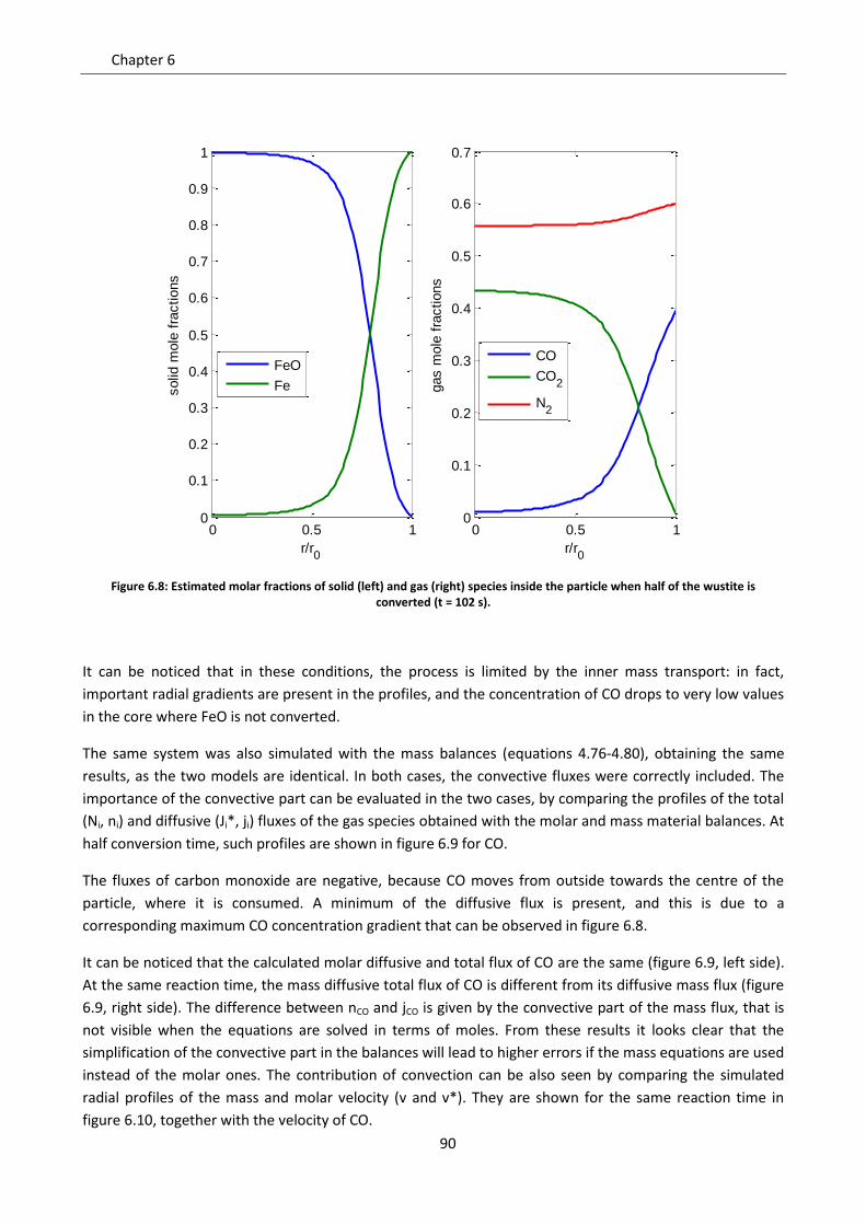
Chapter 6
90
Figure 6.8: Estimated molar fractions of solid (left) and gas (right) species inside the particle when half of the wustite is converted (t = 102 s).
It can be noticed that in these conditions, the process is limited by the inner mass transport: in fact,
important radial gradients are present in the profiles, and the concentration of CO drops to very low values
in the core where FeO is not converted.
The same system was also simulated with the mass balances (equations 4.76-4.80), obtaining the same
results, as the two models are identical. In both cases, the convective fluxes were correctly included. The
importance of the convective part can be evaluated in the two cases, by comparing the profiles of the total
(Ni, ni) and diffusive (Ji*, ji) fluxes of the gas species obtained with the molar and mass material balances. At
half conversion time, such profiles are shown in figure 6.9 for CO.
The fluxes of carbon monoxide are negative, because CO moves from outside towards the centre of the
particle, where it is consumed. A minimum of the diffusive flux is present, and this is due to a
corresponding maximum CO concentration gradient that can be observed in figure 6.8.
It can be noticed that the calculated molar diffusive and total flux of CO are the same (figure 6.9, left side).
At the same reaction time, the mass diffusive total flux of CO is different from its diffusive mass flux (figure
6.9, right side). The difference between nCO and jCO is given by the convective part of the mass flux, that is
not visible when the equations are solved in terms of moles. From these results it looks clear that the
simplification of the convective part in the balances will lead to higher errors if the mass equations are used
instead of the molar ones. The contribution of convection can be also seen by comparing the simulated
radial profiles of the mass and molar velocity (v and v*). They are shown for the same reaction time in
figure 6.10, together with the velocity of CO.
0 0.5 10
0.1
0.2
0.3
0.4
0.5
0.6
0.7
0.8
0.9
1
r/r0
solid
mole
fra
ctions
FeO
Fe
0 0.5 10
0.1
0.2
0.3
0.4
0.5
0.6
0.7
r/r0
gas m
ole
fra
ctions
CO
CO2
N2
Role of diffusion and convection in particle models
91
Figure 6.9: Diffusive and total (diffusive + convective) fluxes of CO at half conversion time (t = 102 s) inside the particle. Molar fluxes (left) and mass fluxes (right).
Figure 6.10: Radial profiles of the mass gas velocity (v), molar gas velocity (v*) and velocity of CO at half conversion time (t = 102 s). Results in linear scale (left), and logarithmic scale of their absolute values (right).
0 0.5 1-2
-1.8
-1.6
-1.4
-1.2
-1
-0.8
-0.6
-0.4
-0.2
0x 10
-5
r/r0
Mola
r fluxes (
mol/cm
2s)
J*CO
NCO
0 0.5 1-7
-6
-5
-4
-3
-2
-1
0
1x 10
-4
r/r0
Mass f
luxes (
g/c
m2s)
jCO
nCO
0 0.2 0.4 0.6 0.8 1-8
-7
-6
-5
-4
-3
-2
-1
0
1
r/r0
velo
city (
cm
/s)
v
v*
vCO
0 0.2 0.4 0.6 0.8 110
-10
10-8
10-6
10-4
10-2
100
102
r/r0
absolu
te v
elo
city (
cm
/s)
v
v*
vCO
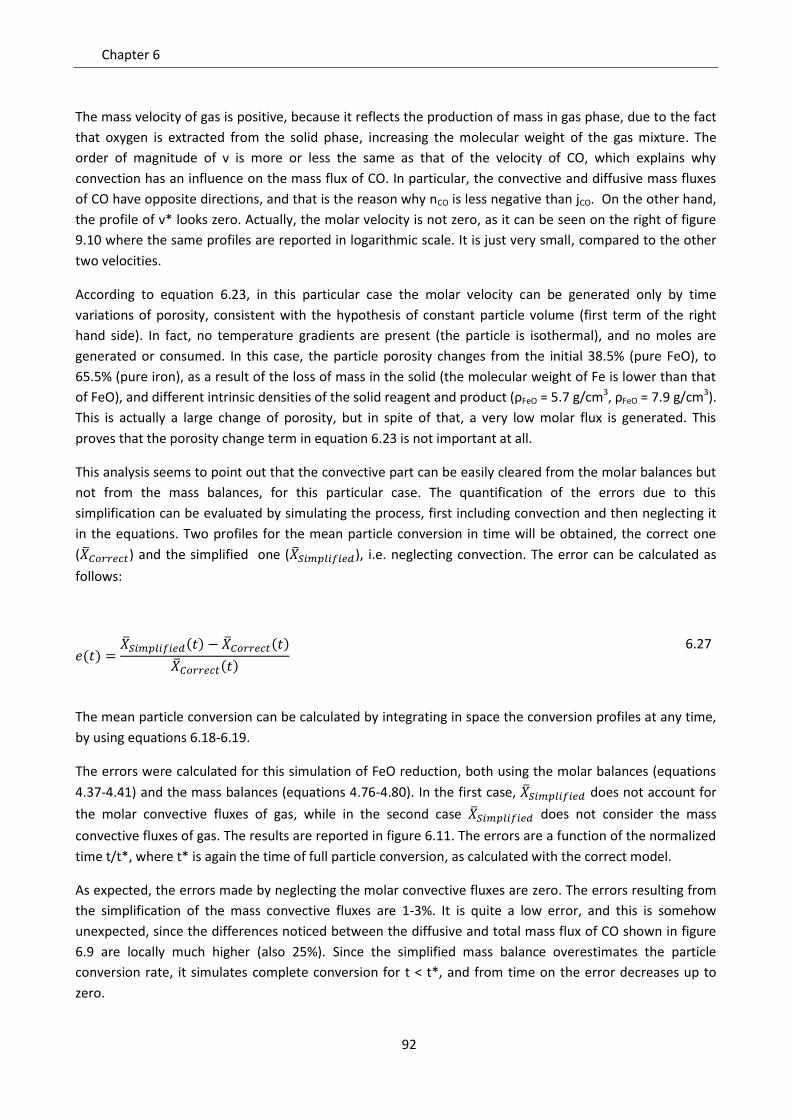
Chapter 6
92
The mass velocity of gas is positive, because it reflects the production of mass in gas phase, due to the fact
that oxygen is extracted from the solid phase, increasing the molecular weight of the gas mixture. The
order of magnitude of v is more or less the same as that of the velocity of CO, which explains why
convection has an influence on the mass flux of CO. In particular, the convective and diffusive mass fluxes
of CO have opposite directions, and that is the reason why nCO is less negative than jCO. On the other hand,
the profile of v* looks zero. Actually, the molar velocity is not zero, as it can be seen on the right of figure
9.10 where the same profiles are reported in logarithmic scale. It is just very small, compared to the other
two velocities.
According to equation 6.23, in this particular case the molar velocity can be generated only by time
variations of porosity, consistent with the hypothesis of constant particle volume (first term of the right
hand side). In fact, no temperature gradients are present (the particle is isothermal), and no moles are
generated or consumed. In this case, the particle porosity changes from the initial 38.5% (pure FeO), to
65.5% (pure iron), as a result of the loss of mass in the solid (the molecular weight of Fe is lower than that
of FeO), and different intrinsic densities of the solid reagent and product (ρFeO = 5.7 g/cm3, ρFeO = 7.9 g/cm3).
This is actually a large change of porosity, but in spite of that, a very low molar flux is generated. This
proves that the porosity change term in equation 6.23 is not important at all.
This analysis seems to point out that the convective part can be easily cleared from the molar balances but
not from the mass balances, for this particular case. The quantification of the errors due to this
simplification can be evaluated by simulating the process, first including convection and then neglecting it
in the equations. Two profiles for the mean particle conversion in time will be obtained, the correct one
( ) and the simplified one ( ), i.e. neglecting convection. The error can be calculated as
follows:
6.27
The mean particle conversion can be calculated by integrating in space the conversion profiles at any time,
by using equations 6.18-6.19.
The errors were calculated for this simulation of FeO reduction, both using the molar balances (equations
4.37-4.41) and the mass balances (equations 4.76-4.80). In the first case, does not account for
the molar convective fluxes of gas, while in the second case does not consider the mass
convective fluxes of gas. The results are reported in figure 6.11. The errors are a function of the normalized
time t/t*, where t* is again the time of full particle conversion, as calculated with the correct model.
As expected, the errors made by neglecting the molar convective fluxes are zero. The errors resulting from
the simplification of the mass convective fluxes are 1-3%. It is quite a low error, and this is somehow
unexpected, since the differences noticed between the diffusive and total mass flux of CO shown in figure
6.9 are locally much higher (also 25%). Since the simplified mass balance overestimates the particle
conversion rate, it simulates complete conversion for t < t*, and from time on the error decreases up to
zero.
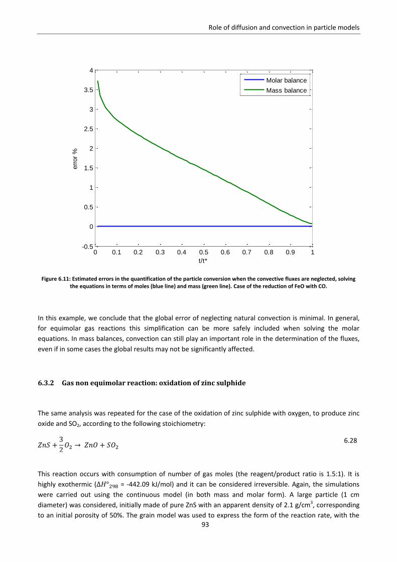
Role of diffusion and convection in particle models
93
Figure 6.11: Estimated errors in the quantification of the particle conversion when the convective fluxes are neglected, solving the equations in terms of moles (blue line) and mass (green line). Case of the reduction of FeO with CO.
In this example, we conclude that the global error of neglecting natural convection is minimal. In general,
for equimolar gas reactions this simplification can be more safely included when solving the molar
equations. In mass balances, convection can still play an important role in the determination of the fluxes,
even if in some cases the global results may not be significantly affected.
6.3.2 Gas non equimolar reaction: oxidation of zinc sulphide
The same analysis was repeated for the case of the oxidation of zinc sulphide with oxygen, to produce zinc
oxide and SO2, according to the following stoichiometry:
6.28
This reaction occurs with consumption of number of gas moles (the reagent/product ratio is 1.5:1). It is
highly exothermic ( = -442.09 kJ/mol) and it can be considered irreversible. Again, the simulations
were carried out using the continuous model (in both mass and molar form). A large particle (1 cm
diameter) was considered, initially made of pure ZnS with an apparent density of 2.1 g/cm3, corresponding
to an initial porosity of 50%. The grain model was used to express the form of the reaction rate, with the
0 0.1 0.2 0.3 0.4 0.5 0.6 0.7 0.8 0.9 1-0.5
0
0.5
1
1.5
2
2.5
3
3.5
4
t/t*
err
or
%
Molar balance
Mass balance
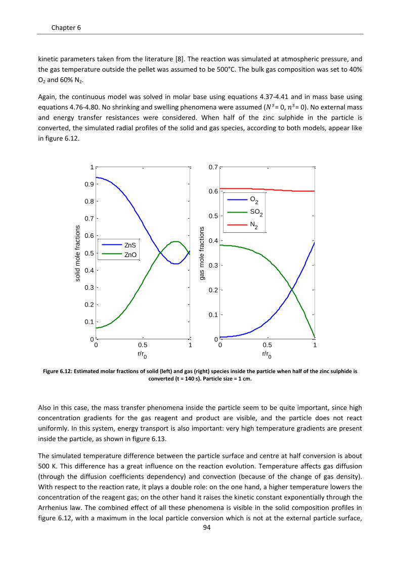
Chapter 6
94
kinetic parameters taken from the literature [8]. The reaction was simulated at atmospheric pressure, and
the gas temperature outside the pellet was assumed to be 500°C. The bulk gas composition was set to 40%
O2 and 60% N2.
Again, the continuous model was solved in molar base using equations 4.37-4.41 and in mass base using
equations 4.76-4.80. No shrinking and swelling phenomena were assumed ( = 0, = 0). No external mass
and energy transfer resistances were considered. When half of the zinc sulphide in the particle is
converted, the simulated radial profiles of the solid and gas species, according to both models, appear like
in figure 6.12.
Figure 6.12: Estimated molar fractions of solid (left) and gas (right) species inside the particle when half of the zinc sulphide is converted (t = 140 s). Particle size = 1 cm.
Also in this case, the mass transfer phenomena inside the particle seem to be quite important, since high
concentration gradients for the gas reagent and product are visible, and the particle does not react
uniformly. In this system, energy transport is also important: very high temperature gradients are present
inside the particle, as shown in figure 6.13.
The simulated temperature difference between the particle surface and centre at half conversion is about
500 K. This difference has a great influence on the reaction evolution. Temperature affects gas diffusion
(through the diffusion coefficients dependency) and convection (because of the change of gas density).
With respect to the reaction rate, it plays a double role: on the one hand, a higher temperature lowers the
concentration of the reagent gas; on the other hand it raises the kinetic constant exponentially through the
Arrhenius law. The combined effect of all these phenomena is visible in the solid composition profiles in
figure 6.12, with a maximum in the local particle conversion which is not at the external particle surface,
0 0.5 10
0.1
0.2
0.3
0.4
0.5
0.6
0.7
0.8
0.9
1
r/r0
solid
mole
fra
ctions
ZnS
ZnO
0 0.5 10
0.1
0.2
0.3
0.4
0.5
0.6
0.7
r/r0
gas m
ole
fra
ctions
O2
SO2
N2
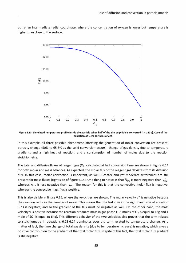
Role of diffusion and convection in particle models
95
but at an intermediate radial coordinate, where the concentration of oxygen is lower but temperature is
higher than close to the surface.
Figure 6.13: Simulated temperature profile inside the particle when half of the zinc sulphide is converted (t = 140 s). Case of the oxidation of 1 cm particles of ZnS
In this example, all three possible phenomena affecting the generation of molar convection are present:
porosity change (50% to 65.5% as the solid conversion occurs), change of gas density due to temperature
gradients and a high heat of reaction, and a consumption of number of moles due to the reaction
stoichiometry.
The total and diffusive fluxes of reagent gas (O2) calculated at half conversion time are shown in figure 6.14
for both molar and mass balances. As expected, the molar flux of the reagent gas deviates from its diffusion
flux. In this case, molar convection is important, as well. Greater and yet moderate differences are still
present for mass fluxes (right side of figure 6.14). One thing to notice is that is more negative than ,
whereas is less negative than . The reason for this is that the convective molar flux is negative,
whereas the convective mass flux is positive.
This is also visible in figure 6.15, where the velocities are shown. The molar velocity v* is negative because
the reaction reduces the number of moles. This means that the last sum in the right hand side of equation
6.23 is negative, and so the gradient of the flux must be negative as well. On the other hand, the mass
velocity v is positive because the reaction produces mass in gas phase (1.5 moles of O2 is equal to 48g and 1
mole of SO2 is equal to 64g). This different behavior of the two velocities also proves that the term related
to stoichiometry in equations 6.23-6.24 dominates over the term related to temperature change. As a
matter of fact, the time change of total gas density (due to temperature increase) is negative, which gives a
positive contribution to the gradient of the total molar flux. In spite of this fact, the total molar flux gradient
is still negative.
0 0.1 0.2 0.3 0.4 0.5 0.6 0.7 0.8 0.9 1700
800
900
1000
1100
1200
1300
r/r0
T (
K)
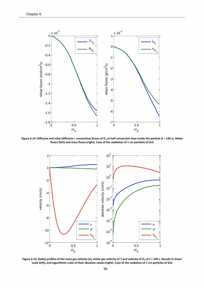
Chapter 6
96
Figure 6.14: Diffusive and total (diffusive + convective) fluxes of O2 at half conversion time inside the particle (t = 140 s). Molar fluxes (left) and mass fluxes (right). Case of the oxidation of 1 cm particles of ZnS
Figure 6.15: Radial profiles of the mass gas velocity (v), molar gas velocity (v*) and velocity of O2 at t = 140 s. Results in linear scale (left), and logarithmic scale of their absolute values (right). Case of the oxidation of 1 cm particles of ZnS
0 0.5 1-1.8
-1.6
-1.4
-1.2
-1
-0.8
-0.6
-0.4
-0.2
0x 10
-5
r/r0
Mola
r fluxes (
mol/cm
2s)
J*O
2
NO
2
0 0.5 1-7
-6
-5
-4
-3
-2
-1
0
1x 10
-4
r/r0
Mass f
luxes (
g/c
m2s)
jO
2
nO
2
0 0.5 1-12
-10
-8
-6
-4
-2
0
2
r/r0
velo
city (
cm
/s)
v
v*
vO
2
0 0.5 110
-6
10-5
10-4
10-3
10-2
10-1
100
101
102
r/r0
absolu
te v
elo
city (
cm
/s)
v
v*
vO
2
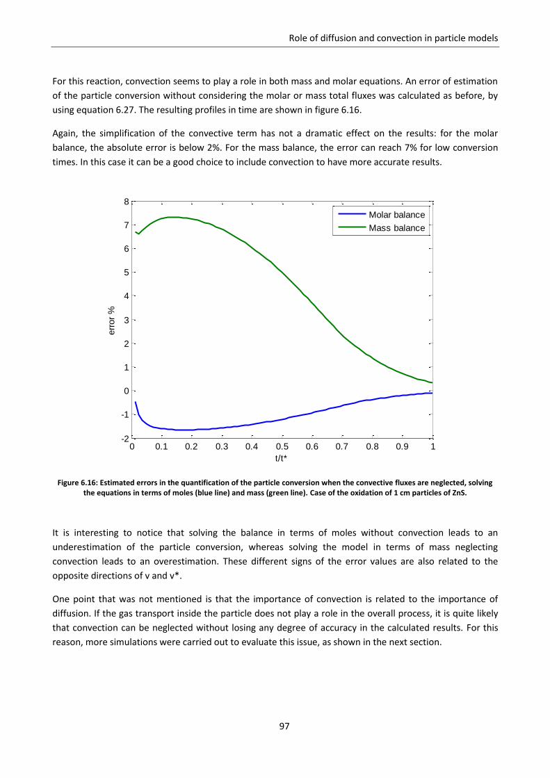
Role of diffusion and convection in particle models
97
For this reaction, convection seems to play a role in both mass and molar equations. An error of estimation
of the particle conversion without considering the molar or mass total fluxes was calculated as before, by
using equation 6.27. The resulting profiles in time are shown in figure 6.16.
Again, the simplification of the convective term has not a dramatic effect on the results: for the molar
balance, the absolute error is below 2%. For the mass balance, the error can reach 7% for low conversion
times. In this case it can be a good choice to include convection to have more accurate results.
Figure 6.16: Estimated errors in the quantification of the particle conversion when the convective fluxes are neglected, solving the equations in terms of moles (blue line) and mass (green line). Case of the oxidation of 1 cm particles of ZnS.
It is interesting to notice that solving the balance in terms of moles without convection leads to an
underestimation of the particle conversion, whereas solving the model in terms of mass neglecting
convection leads to an overestimation. These different signs of the error values are also related to the
opposite directions of v and v*.
One point that was not mentioned is that the importance of convection is related to the importance of
diffusion. If the gas transport inside the particle does not play a role in the overall process, it is quite likely
that convection can be neglected without losing any degree of accuracy in the calculated results. For this
reason, more simulations were carried out to evaluate this issue, as shown in the next section.
0 0.1 0.2 0.3 0.4 0.5 0.6 0.7 0.8 0.9 1-2
-1
0
1
2
3
4
5
6
7
8
t/t*
err
or
%
Molar balance
Mass balance
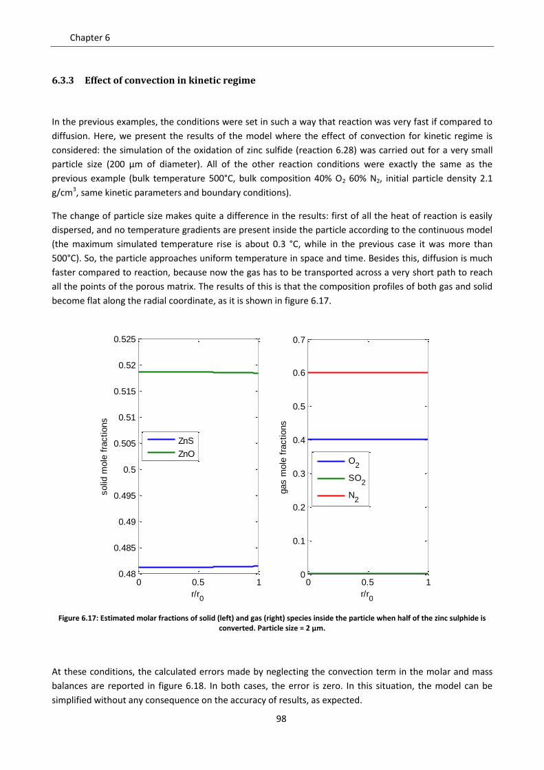
Chapter 6
98
6.3.3 Effect of convection in kinetic regime
In the previous examples, the conditions were set in such a way that reaction was very fast if compared to
diffusion. Here, we present the results of the model where the effect of convection for kinetic regime is
considered: the simulation of the oxidation of zinc sulfide (reaction 6.28) was carried out for a very small
particle size (200 µm of diameter). All of the other reaction conditions were exactly the same as the
previous example (bulk temperature 500°C, bulk composition 40% O2 60% N2, initial particle density 2.1
g/cm3, same kinetic parameters and boundary conditions).
The change of particle size makes quite a difference in the results: first of all the heat of reaction is easily
dispersed, and no temperature gradients are present inside the particle according to the continuous model
(the maximum simulated temperature rise is about 0.3 °C, while in the previous case it was more than
500°C). So, the particle approaches uniform temperature in space and time. Besides this, diffusion is much
faster compared to reaction, because now the gas has to be transported across a very short path to reach
all the points of the porous matrix. The results of this is that the composition profiles of both gas and solid
become flat along the radial coordinate, as it is shown in figure 6.17.
Figure 6.17: Estimated molar fractions of solid (left) and gas (right) species inside the particle when half of the zinc sulphide is converted. Particle size = 2 µm.
At these conditions, the calculated errors made by neglecting the convection term in the molar and mass
balances are reported in figure 6.18. In both cases, the error is zero. In this situation, the model can be
simplified without any consequence on the accuracy of results, as expected.
0 0.5 10.48
0.485
0.49
0.495
0.5
0.505
0.51
0.515
0.52
0.525
r/r0
solid
mole
fra
ctions
ZnS
ZnO
0 0.5 10
0.1
0.2
0.3
0.4
0.5
0.6
0.7
r/r0
gas m
ole
fra
ctions
O2
SO2
N2
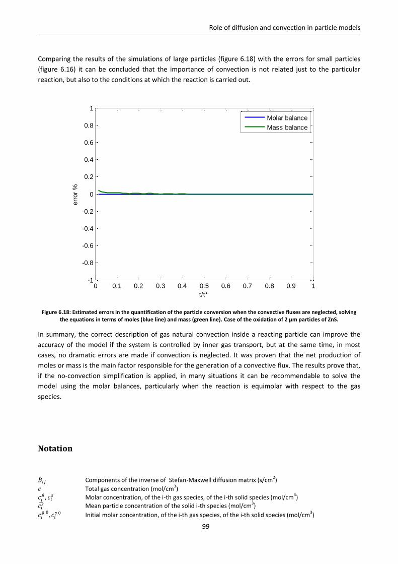
Role of diffusion and convection in particle models
99
Comparing the results of the simulations of large particles (figure 6.18) with the errors for small particles
(figure 6.16) it can be concluded that the importance of convection is not related just to the particular
reaction, but also to the conditions at which the reaction is carried out.
Figure 6.18: Estimated errors in the quantification of the particle conversion when the convective fluxes are neglected, solving the equations in terms of moles (blue line) and mass (green line). Case of the oxidation of 2 µm particles of ZnS.
In summary, the correct description of gas natural convection inside a reacting particle can improve the
accuracy of the model if the system is controlled by inner gas transport, but at the same time, in most
cases, no dramatic errors are made if convection is neglected. It was proven that the net production of
moles or mass is the main factor responsible for the generation of a convective flux. The results prove that,
if the no-convection simplification is applied, in many situations it can be recommendable to solve the
model using the molar balances, particularly when the reaction is equimolar with respect to the gas
species.
Notation
Components of the inverse of Stefan-Maxwell diffusion matrix (s/cm2)
Total gas concentration (mol/cm3)
Molar concentration, of the i-th gas species, of the i-th solid species (mol/cm3)
Mean particle concentration of the solid i-th species (mol/cm
3)
Initial molar concentration, of the i-th gas species, of the i-th solid species (mol/cm
3)
0 0.1 0.2 0.3 0.4 0.5 0.6 0.7 0.8 0.9 1-1
-0.8
-0.6
-0.4
-0.2
0
0.2
0.4
0.6
0.8
1
t/t*
err
or
%
Molar balance
Mass balance
Chapter 6
100
Concentration of the i-th gas species outside the particle, in bulk phase (mol/cm3)
Total concentration of gas phase, of solid phase (mol/cm3)
Multicomponent diffusion coefficient of i in j (cm2/s)
Components of the Stefan-Maxwell diffusion matrix (cm2/s)
Diffusion coefficients of i in the gas mixture, for the molar fluxes (cm2/s)
Relative error of estimation of the particle conversion neglecting gas convection Relative error of estimation of the particle conversion with Fick’s law Relative error of estimation of the particle conversion with Mixture averaged model Molar diffusive flux of i (mol/cm
2/s)
volumetric kinetic constant (1/s) Molecular weight of the i-th species (g/mol) Molecular weight of gas phase (g/mol) Number of gas species in the system Total molar flux of the gas phase (mol/cm
2/s)
Total mass flux of the gas phase (g/cm2/s)
P Pressure (Pa) Particle radius (cm) Radial coordinate (cm)
Molar source term for the i-th gas species, for the i-th solid species (mol/cm3/s )
Absolute temperature (K) t Time (s) Velocity of the i-th species (cm/s) Velocity of the gas center of mass (cm/s) Velocity of the gas molar center of mass (cm/s) Conversion of the i-th solid phase
Mean particle conversion Mean particle conversion calculated with Fick, Mixture averaged, Stefan Maxwell models Mean particle conversion calculated including convection Mean particle conversion calculated neglecting convection
Molar fraction of the i-th gas species Mass fraction of the i-th gas species Greek letters ԑ Porosity Thiele modulus Mass density of the gas phase (g/cm
3)
101
Chapter 7. Particle models for Chemical Looping Combustion
In the previous sections, continuous models have been studied in general, with respect to the contribution
of the kinetic and intra particle mass transport phenomena. In practical applications, to achieve a reliable
description of the evolution of the particle one of the key issues comes from correctly describing the
influence of the particle morphology evolution (i.e. porosity field, superficial area) to the reaction and gas
diffusion terms inside the balance equations. The evolution of particle morphology is often related to the
particular process, and reaction conditions used, so it must be studied ad hoc. As a matter of fact, the
available experimental data on the particle conversion in time can be usually explained with the same
degree of accuracy by assuming different hypotheses, that need to be verified by carefully characterizing
the solid particle.
In this section, this issue is discussed, by considering the application of the continuous model to chemical
looping combustion processes. This has been possible thanks to the collaboration with the Technical
University of Eindhoven (TU/e), in particular with the multiphase reactors research group.
7.1 Chemical Looping Combustion
Chemical looping combustion (CLC) derives from the interest in the control and treatment of emissions of
gases in chemical processes. This is increasing more and more, and new sustainable technologies must be
developed in order to accomplish this goal. In such a context, chemical looping combustion is a new
process that can combine the need to get energy from conventional fossil fuels with the possibility of
treating the produced gases in a better and more efficient way, also with respect to the coupling with CO2
capture techniques. The main advantage of CLC is that the fuel and oxygen are never mixed up in a single
gas phase: all the reactions involving oxygen actually occur via a solid oxygen carrier, which is constantly
regenerated.
A general scheme of a chemical looping combustion process is shown in Figure 7.1. Two reactors are
needed: in the first one, air is fluxed in a moving or fluidized bed where a metal compound is oxidized. The
discharged gas is made of air, depleted of oxygen. This step is always exothermic, and provides the energy
requested by the process. The oxidized solid is then moved to a second reactor, where it is in contact with
the gas fuel. In this unit, the solid is reduced back to its original state and can be recycled to the first
reactor. The outlet gas is generally composed of CO2 and H2O that can be easily separated by steam
condensation, obtaining pure streams. The second step can be endothermic, with the heat of reaction that
can be provided by the oxidation step. The global reaction of the whole process is the gas fuel oxidation,
whereas the solid carrier is never consumed, theoretically. In synthesis, Chemical looping Combustion
provides CO2 separation in itself.
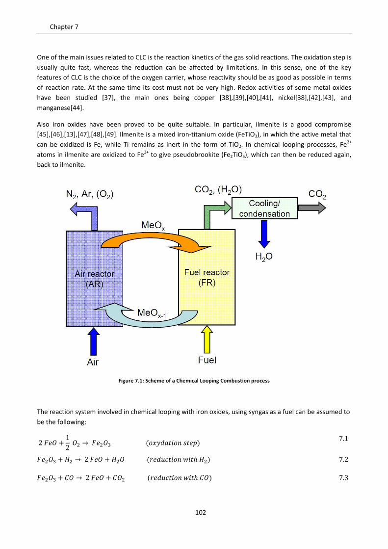
Chapter 7
102
One of the main issues related to CLC is the reaction kinetics of the gas solid reactions. The oxidation step is
usually quite fast, whereas the reduction can be affected by limitations. In this sense, one of the key
features of CLC is the choice of the oxygen carrier, whose reactivity should be as good as possible in terms
of reaction rate. At the same time its cost must not be very high. Redox activities of some metal oxides
have been studied [37], the main ones being copper [38],[39],[40],[41], nickel[38],[42],[43], and
manganese[44].
Also iron oxides have been proved to be quite suitable. In particular, ilmenite is a good compromise
[45],[46],[13],[47],[48],[49]. Ilmenite is a mixed iron-titanium oxide (FeTiO3), in which the active metal that
can be oxidized is Fe, while Ti remains as inert in the form of TiO2. In chemical looping processes, Fe2+
atoms in ilmenite are oxidized to Fe3+ to give pseudobrookite (Fe2TiO5), which can then be reduced again,
back to ilmenite.
Figure 7.1: Scheme of a Chemical Looping Combustion process
The reaction system involved in chemical looping with iron oxides, using syngas as a fuel can be assumed to
be the following:
7.1
7.2
7.3
Particle models for Chemical Looping Combustion
103
The sum of reactions 7.1 and 7.2 is the reaction of combustion of hydrogen, whereas the sum of 7.1 and 7.3
is the combustion of carbon monoxide:
7.4
7.5
In CLC processes, the same solid pellets are involved in a high number of oxidation-reaction cycles, usually
at high temperature. This may have an influence on the internal structure of the particles, that can change
in time within a single cycle and along cycles.
Within CLC processes, both simple shrinking core models and continuous models are used in the literature.
A shrinking-core model approach was followed by Abad et al. [13], to study the kinetics of the ilmenite-
pseudobrookite system, for both oxidation and reduction steps. Noorman et al. [50] proposed a detailed
model to describe Cu/CuO redox behavior in chemical looping, evaluating the contribution of internal and
external mass transfer with respect to chemical reactions. Zhou et al. [51] developed a kinetic scheme for
Ni/NiO CLC systems based on the grain model, and applied a continuous particle model to a fixed bed
chemical looping reactor model [52].
7.2 Experimental estimation of carriers reactivity: TGA analysis
An important characteristic parameter of the solid species involved in CLC is the oxygen carrier capacity RO,
which defines the amount of oxygen that the carrier can transport due to the oxidation reduction loop, per
unit of mass of oxidized sample:
7.6
This quantity is fixed for any oxygen carrier, and it is related to the reaction stoichiometry of the single step,
and also to the mass of non reacting solid phase (for instance rutile, in the case of the ilmenite-
pseudobrookite system). The mass of the oxidized solid is always greater than that of the reduced one, and
in general RO should be as high as possible. At the same time, a solid conversion X can be related the mass
of the solid sample in any moment of the reaction. For the oxidation step it is as follows:
7.7
In the same way, for the reduction step:
Chapter 7
104
7.8
For a sample made of a single spherical particle, can be calculated by the continuous model by
considering the integrals in space of the solid species concentrations. With reference to the solution of the
set of equations 4.37-4.41, the particle mass is:
7.9
Consistently, and can result from equation 7.9 for zero and infinite reaction times of the
reduction step, respectively. If the system is made of more particles, all reacting in the same way (the gas
composition outside each particle is the same), the calculated conversion of the group of particles is the
same as the one calculated for a single particle.
This way of defining conversion is quite useful, because can also be easily measured experimentally,
by performing the gas solid reactions in thermo gravimetric (TGA) setups. Thermo gravimetric analysis is a
technique that involves the accurate measurement of the weight of a sample, changing in time,
corresponding to an assigned temperature profile. In this way, physical and or chemical modifications of
the sample can be detected and quantified. The experimental setup is made of a balance, connected to a
crucible where the sample is placed, which is inside a programmable furnace where the desired
temperature is set. In many setups, the TGA apparatus can also be used as a reactor, with a gas being
constantly fed into the furnace and reacting with the sample on the balance. In this sense the loss or gain in
weight of the sample in time can be related to the kinetics of a chemical reaction.
In order to study chemical looping processes, TGA is quite useful, because the same sample of oxygen
carrier can be used to evaluate the oxidation and reduction steps, by alternately feeding air and fuel to the
balance where the carrier is placed. By knowing the weight of the fully reduced and fully oxidized sample,
the conversions of equation 7.7 and 7.8 can then be measured. So TGA provides global quantitative data
about the solid particle conversion, that can be easily compared with the results of a particle model.
Figure 7.2 shows an example of experimental data obtained by the laboratories of Tu\E by reducing
particles of pseudobrookite (Fe2TiO5). A sample of about 100 mg of small particles (about 200 µm of
diameter) was placed on the thermo balance crucible. In this example, CO is used as a reducing agent, and
in all three cases the fed gas is composed of 15% CO and 20% CO2 in nitrogen. A quite high gas flow rate
was provided (about 500 mL/min) in order to avoid external mass transfer limitations as much as possible.
The profiles show the experimental particles conversion at three fixed temperatures (600°C, 700°C and
800°C) and atmospheric pressure. The conversion profiles are the result of the reduction of iron oxide
present in the particle, according to reaction 7.3.
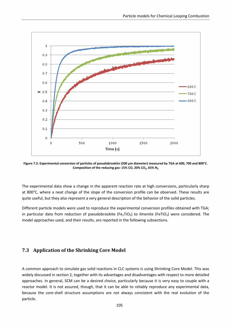
Particle models for Chemical Looping Combustion
105
Figure 7.2: Experimental conversion of particles of pseudobrookite (200 µm diameter) measured by TGA at 600, 700 and 800°C. Composition of the reducing gas: 15% CO, 20% CO2, 65% N2
The experimental data show a change in the apparent reaction rate at high conversions, particularly sharp
at 800°C, where a neat change of the slope of the conversion profile can be observed. These results are
quite useful, but they also represent a very general description of the behavior of the solid particles.
Different particle models were used to reproduce the experimental conversion profiles obtained with TGA;
in particular data from reduction of pseudobrookite (Fe2TiO5) to ilmenite (FeTiO3) were considered. The
model approaches used, and their results, are reported in the following subsections.
7.3 Application of the Shrinking Core Model
A common approach to simulate gas solid reactions in CLC systems is using Shrinking Core Model. This was
widely discussed in section 2, together with its advantages and disadvantages with respect to more detailed
approaches. In general, SCM can be a desired choice, particularly because it is very easy to couple with a
reactor model. It is not assured, though, that it can be able to reliably reproduce any experimental data,
because the core-shell structure assumptions are not always consistent with the real evolution of the
particle.
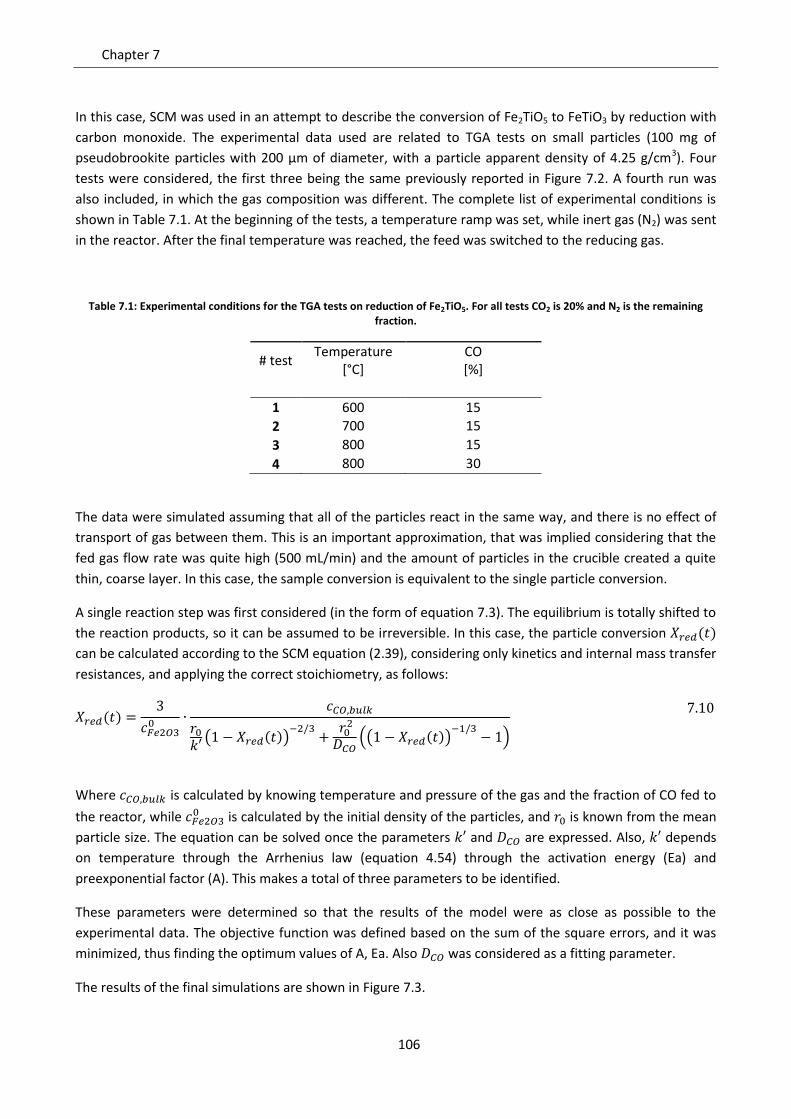
Chapter 7
106
In this case, SCM was used in an attempt to describe the conversion of Fe2TiO5 to FeTiO3 by reduction with
carbon monoxide. The experimental data used are related to TGA tests on small particles (100 mg of
pseudobrookite particles with 200 µm of diameter, with a particle apparent density of 4.25 g/cm3). Four
tests were considered, the first three being the same previously reported in Figure 7.2. A fourth run was
also included, in which the gas composition was different. The complete list of experimental conditions is
shown in Table 7.1. At the beginning of the tests, a temperature ramp was set, while inert gas (N2) was sent
in the reactor. After the final temperature was reached, the feed was switched to the reducing gas.
Table 7.1: Experimental conditions for the TGA tests on reduction of Fe2TiO5. For all tests CO2 is 20% and N2 is the remaining fraction.
# test Temperature
[°C] CO [%]
1 600 15
2 700 15
3 800 15
4 800 30
The data were simulated assuming that all of the particles react in the same way, and there is no effect of
transport of gas between them. This is an important approximation, that was implied considering that the
fed gas flow rate was quite high (500 mL/min) and the amount of particles in the crucible created a quite
thin, coarse layer. In this case, the sample conversion is equivalent to the single particle conversion.
A single reaction step was first considered (in the form of equation 7.3). The equilibrium is totally shifted to
the reaction products, so it can be assumed to be irreversible. In this case, the particle conversion
can be calculated according to the SCM equation (2.39), considering only kinetics and internal mass transfer
resistances, and applying the correct stoichiometry, as follows:
7.10
Where is calculated by knowing temperature and pressure of the gas and the fraction of CO fed to
the reactor, while is calculated by the initial density of the particles, and is known from the mean
particle size. The equation can be solved once the parameters and are expressed. Also, depends
on temperature through the Arrhenius law (equation 4.54) through the activation energy (Ea) and
preexponential factor (A). This makes a total of three parameters to be identified.
These parameters were determined so that the results of the model were as close as possible to the
experimental data. The objective function was defined based on the sum of the square errors, and it was
minimized, thus finding the optimum values of A, Ea. Also was considered as a fitting parameter.
The results of the final simulations are shown in Figure 7.3.
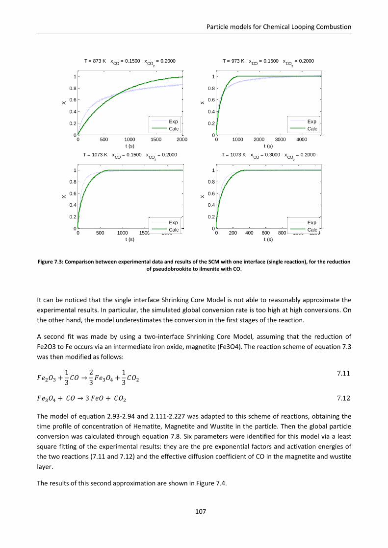
Particle models for Chemical Looping Combustion
107
Figure 7.3: Comparison between experimental data and results of the SCM with one interface (single reaction), for the reduction of pseudobrookite to ilmenite with CO.
It can be noticed that the single interface Shrinking Core Model is not able to reasonably approximate the
experimental results. In particular, the simulated global conversion rate is too high at high conversions. On
the other hand, the model underestimates the conversion in the first stages of the reaction.
A second fit was made by using a two-interface Shrinking Core Model, assuming that the reduction of
Fe2O3 to Fe occurs via an intermediate iron oxide, magnetite (Fe3O4). The reaction scheme of equation 7.3
was then modified as follows:
7.11
7.12
The model of equation 2.93-2.94 and 2.111-2.227 was adapted to this scheme of reactions, obtaining the
time profile of concentration of Hematite, Magnetite and Wustite in the particle. Then the global particle
conversion was calculated through equation 7.8. Six parameters were identified for this model via a least
square fitting of the experimental results: they are the pre exponential factors and activation energies of
the two reactions (7.11 and 7.12) and the effective diffusion coefficient of CO in the magnetite and wustite
layer.
The results of this second approximation are shown in Figure 7.4.
0 500 1000 1500 20000
0.2
0.4
0.6
0.8
1
T = 873 K xCO
= 0.1500 xCO
2
= 0.2000
t (s)
X
0 1000 2000 3000 40000
0.2
0.4
0.6
0.8
1
T = 973 K xCO
= 0.1500 xCO
2
= 0.2000
t (s)
X
0 500 1000 1500 20000
0.2
0.4
0.6
0.8
1
T = 1073 K xCO
= 0.1500 xCO
2
= 0.2000
t (s)
X
0 200 400 600 800 1000 12000
0.2
0.4
0.6
0.8
1
T = 1073 K xCO
= 0.3000 xCO
2
= 0.2000
t (s)
X
Exp
Calc
Exp
Calc
Exp
Calc
Exp
Calc
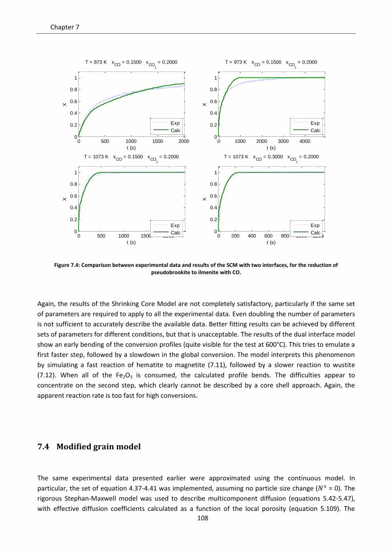
Chapter 7
108
Figure 7.4: Comparison between experimental data and results of the SCM with two interfaces, for the reduction of pseudobrookite to ilmenite with CO.
Again, the results of the Shrinking Core Model are not completely satisfactory, particularly if the same set
of parameters are required to apply to all the experimental data. Even doubling the number of parameters
is not sufficient to accurately describe the available data. Better fitting results can be achieved by different
sets of parameters for different conditions, but that is unacceptable. The results of the dual interface model
show an early bending of the conversion profiles (quite visible for the test at 600°C). This tries to emulate a
first faster step, followed by a slowdown in the global conversion. The model interprets this phenomenon
by simulating a fast reaction of hematite to magnetite (7.11), followed by a slower reaction to wustite
(7.12). When all of the Fe2O3 is consumed, the calculated profile bends. The difficulties appear to
concentrate on the second step, which clearly cannot be described by a core shell approach. Again, the
apparent reaction rate is too fast for high conversions.
7.4 Modified grain model
The same experimental data presented earlier were approximated using the continuous model. In
particular, the set of equation 4.37-4.41 was implemented, assuming no particle size change ( = 0). The
rigorous Stephan-Maxwell model was used to describe multicomponent diffusion (equations 5.42-5.47),
with effective diffusion coefficients calculated as a function of the local porosity (equation 5.109). The
0 500 1000 1500 20000
0.2
0.4
0.6
0.8
1
T = 873 K xCO
= 0.1500 xCO
2
= 0.2000
t (s)
X
Exp
Calc
0 1000 2000 3000 40000
0.2
0.4
0.6
0.8
1
T = 973 K xCO
= 0.1500 xCO
2
= 0.2000
t (s)
X
Exp
Calc
0 500 1000 1500 20000
0.2
0.4
0.6
0.8
1
T = 1073 K xCO
= 0.1500 xCO
2
= 0.2000
t (s)
X
Exp
Calc0 200 400 600 800 1000 1200
0
0.2
0.4
0.6
0.8
1
T = 1073 K xCO
= 0.3000 xCO
2
= 0.2000
t (s)
X
Exp
Calc
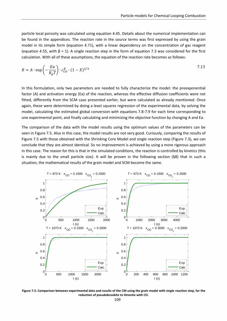
Particle models for Chemical Looping Combustion
109
particle local porosity was calculated using equation 4.45. Details about the numerical implementation can
be found in the appendices. The reaction rate in the source terms was first expressed by using the grain
model in its simple form (equation 4.71), with a linear dependency on the concentration of gas reagent
(equation 4.55, with β = 1). A single reaction step in the form of equation 7.3 was considered for the first
calculation. With all of these assumptions, the equation of the reaction rate becomes as follows:
7.13
In this formulation, only two parameters are needed to fully characterize the model: the preexponential
factor (A) and activation energy (Ea) of the reaction, whereas the effective diffusion coefficients were not
fitted, differently from the SCM case presented earlier, but were calculated as already mentioned. Once
again, these were determined by doing a least squares regression of the experimental data, by solving the
model, calculating the estimated global conversion with equations 7.8-7.9 for each time corresponding to
one experimental point, and finally calculating and minimizing the objective function by changing A and Ea.
The comparison of the data with the model results using the optimum values of the parameters can be
seen in Figure 7.5. Also in this case, the model results are not very good. Curiously, comparing the results of
Figure 7.5 with those obtained with the Shrinking Core Model and single reaction step (Figure 7.3), we can
conclude that they are almost identical. So no improvement is achieved by using a more rigorous approach
in this case. The reason for this is that in the simulated conditions, the reaction is controlled by kinetics (this
is mainly due to the small particle size). It will be proven in the following section (§8) that in such a
situation, the mathematical results of the grain model and SCM become the same.
Figure 7.5: Comparison between experimental data and results of the CM using the grain model with single reaction step, for the reduction of pseudobrookite to ilmenite with CO.
0 500 1000 1500 20000
0.2
0.4
0.6
0.8
1
T = 873 K xCO
= 0.1500 xCO
2
= 0.2000
t (s)
X
Exp
Calc
0 1000 2000 3000 40000
0.2
0.4
0.6
0.8
1
T = 973 K xCO
= 0.1500 xCO
2
= 0.2000
t (s)
X
Exp
Calc
0 500 1000 1500 20000
0.2
0.4
0.6
0.8
1
T = 1073 K xCO
= 0.1500 xCO
2
= 0.2000
t (s)
X
Exp
Calc
0 200 400 600 800 1000 12000
0.2
0.4
0.6
0.8
1
T = 1073 K xCO
= 0.3000 xCO
2
= 0.2000
t (s)
X
Exp
Calc
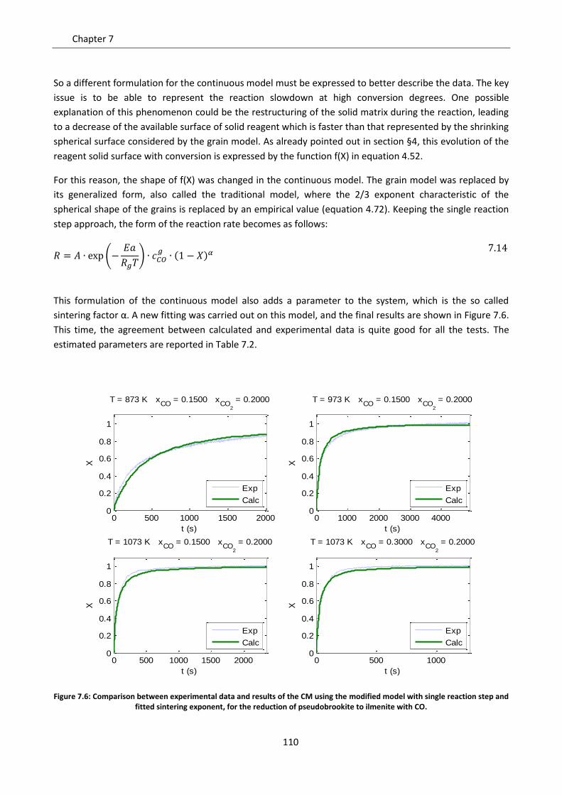
Chapter 7
110
So a different formulation for the continuous model must be expressed to better describe the data. The key
issue is to be able to represent the reaction slowdown at high conversion degrees. One possible
explanation of this phenomenon could be the restructuring of the solid matrix during the reaction, leading
to a decrease of the available surface of solid reagent which is faster than that represented by the shrinking
spherical surface considered by the grain model. As already pointed out in section §4, this evolution of the
reagent solid surface with conversion is expressed by the function f(X) in equation 4.52.
For this reason, the shape of f(X) was changed in the continuous model. The grain model was replaced by
its generalized form, also called the traditional model, where the 2/3 exponent characteristic of the
spherical shape of the grains is replaced by an empirical value (equation 4.72). Keeping the single reaction
step approach, the form of the reaction rate becomes as follows:
7.14
This formulation of the continuous model also adds a parameter to the system, which is the so called
sintering factor α. A new fitting was carried out on this model, and the final results are shown in Figure 7.6.
This time, the agreement between calculated and experimental data is quite good for all the tests. The
estimated parameters are reported in Table 7.2.
Figure 7.6: Comparison between experimental data and results of the CM using the modified model with single reaction step and fitted sintering exponent, for the reduction of pseudobrookite to ilmenite with CO.
0 500 1000 1500 20000
0.2
0.4
0.6
0.8
1
T = 873 K xCO
= 0.1500 xCO
2
= 0.2000
t (s)
X
Exp
Calc
0 1000 2000 3000 40000
0.2
0.4
0.6
0.8
1
T = 973 K xCO
= 0.1500 xCO
2
= 0.2000
t (s)
X
Exp
Calc
0 500 1000 1500 20000
0.2
0.4
0.6
0.8
1
T = 1073 K xCO
= 0.1500 xCO
2
= 0.2000
t (s)
X
Exp
Calc
0 500 10000
0.2
0.4
0.6
0.8
1
T = 1073 K xCO
= 0.3000 xCO
2
= 0.2000
t (s)
X
Exp
Calc
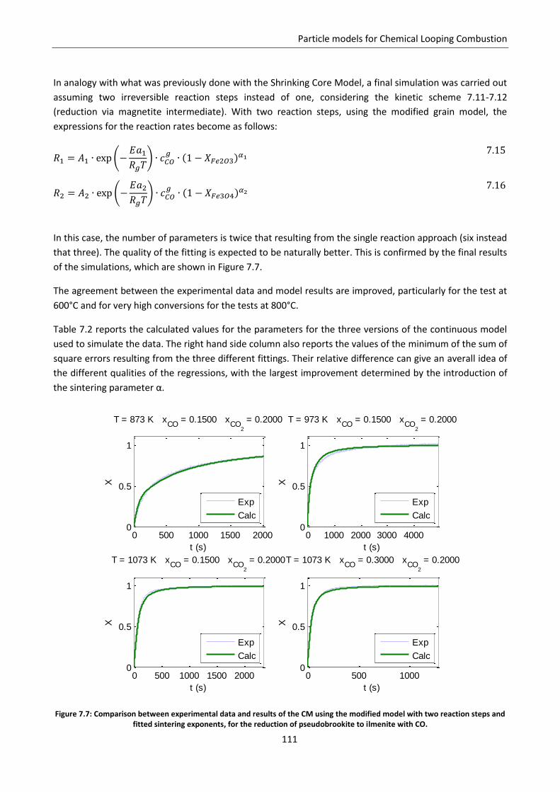
Particle models for Chemical Looping Combustion
111
In analogy with what was previously done with the Shrinking Core Model, a final simulation was carried out
assuming two irreversible reaction steps instead of one, considering the kinetic scheme 7.11-7.12
(reduction via magnetite intermediate). With two reaction steps, using the modified grain model, the
expressions for the reaction rates become as follows:
7.15
7.16
In this case, the number of parameters is twice that resulting from the single reaction approach (six instead
that three). The quality of the fitting is expected to be naturally better. This is confirmed by the final results
of the simulations, which are shown in Figure 7.7.
The agreement between the experimental data and model results are improved, particularly for the test at
600°C and for very high conversions for the tests at 800°C.
Table 7.2 reports the calculated values for the parameters for the three versions of the continuous model
used to simulate the data. The right hand side column also reports the values of the minimum of the sum of
square errors resulting from the three different fittings. Their relative difference can give an averall idea of
the different qualities of the regressions, with the largest improvement determined by the introduction of
the sintering parameter α.
Figure 7.7: Comparison between experimental data and results of the CM using the modified model with two reaction steps and fitted sintering exponents, for the reduction of pseudobrookite to ilmenite with CO.
0 500 1000 1500 20000
0.5
1
T = 873 K xCO
= 0.1500 xCO
2
= 0.2000
t (s)
X
0 1000 2000 3000 40000
0.5
1
T = 973 K xCO
= 0.1500 xCO
2
= 0.2000
t (s)
X
0 500 1000 1500 20000
0.5
1
T = 1073 K xCO
= 0.1500 xCO
2
= 0.2000
t (s)
X
0 500 10000
0.5
1
T = 1073 K xCO
= 0.3000 xCO
2
= 0.2000
t (s)
X
Exp
Calc
Exp
Calc
Exp
Calc
Exp
Calc
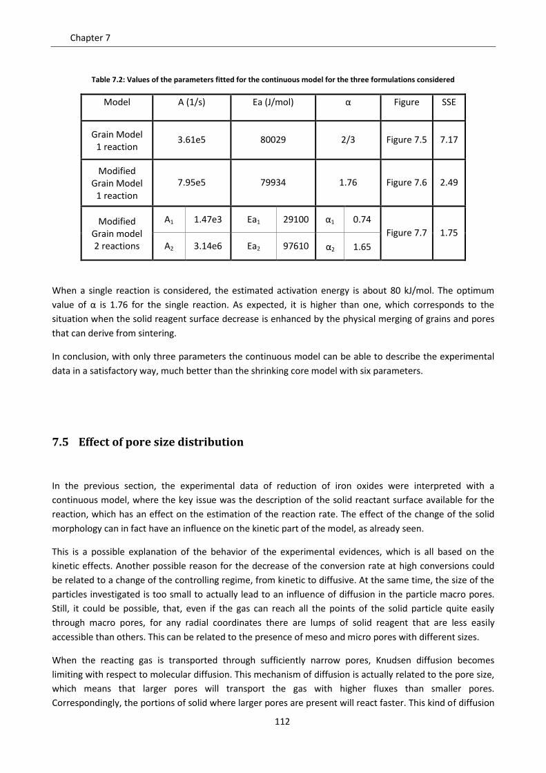
Chapter 7
112
Table 7.2: Values of the parameters fitted for the continuous model for the three formulations considered
Model A (1/s) Ea (J/mol) α Figure SSE
Grain Model 1 reaction
3.61e5 80029 2/3 Figure 7.5 7.17
Modified Grain Model
1 reaction
7.95e5 79934 1.76 Figure 7.6 2.49
Modified Grain model 2 reactions
A1 1.47e3 Ea1 29100 α1 0.74
Figure 7.7 1.75
A2 3.14e6 Ea2 97610 α2 1.65
When a single reaction is considered, the estimated activation energy is about 80 kJ/mol. The optimum
value of α is 1.76 for the single reaction. As expected, it is higher than one, which corresponds to the
situation when the solid reagent surface decrease is enhanced by the physical merging of grains and pores
that can derive from sintering.
In conclusion, with only three parameters the continuous model can be able to describe the experimental
data in a satisfactory way, much better than the shrinking core model with six parameters.
7.5 Effect of pore size distribution
In the previous section, the experimental data of reduction of iron oxides were interpreted with a
continuous model, where the key issue was the description of the solid reactant surface available for the
reaction, which has an effect on the estimation of the reaction rate. The effect of the change of the solid
morphology can in fact have an influence on the kinetic part of the model, as already seen.
This is a possible explanation of the behavior of the experimental evidences, which is all based on the
kinetic effects. Another possible reason for the decrease of the conversion rate at high conversions could
be related to a change of the controlling regime, from kinetic to diffusive. At the same time, the size of the
particles investigated is too small to actually lead to an influence of diffusion in the particle macro pores.
Still, it could be possible, that, even if the gas can reach all the points of the solid particle quite easily
through macro pores, for any radial coordinates there are lumps of solid reagent that are less easily
accessible than others. This can be related to the presence of meso and micro pores with different sizes.
When the reacting gas is transported through sufficiently narrow pores, Knudsen diffusion becomes
limiting with respect to molecular diffusion. This mechanism of diffusion is actually related to the pore size,
which means that larger pores will transport the gas with higher fluxes than smaller pores.
Correspondingly, the portions of solid where larger pores are present will react faster. This kind of diffusion
Particle models for Chemical Looping Combustion
113
resistance occurs on a different scale than that of the radial transport of gas from the outside to the core of
the particle. In fact, large or small micro pores can be present at any radial coordinate. If the transport
through the macro pores is fast but the transport through micro pores is not, in comparison with the rate of
reaction, the particle can still be converted homogeneously along the radial coordinate, but the reaction
rate will decrease in time, as soon as the local portions of solid more easily accessed are consumed, and
only those with smaller micro pores are remaining.
The effect of this decrease depends on the pore size distribution of the particle, that is on the fractions of
solid occupied by any pore size. These can be actually measured for a porous solid, thanks to techniques
based on gas adsorption quantification. This information can thus be translated into the quantification of
the different diffusion resistances that can be present inside the pellets, with a model.
The continuous model presented so far is not able to represent this sub scale. If a single pore size is
assumed, a single value of gas diffusivity is considered inside the particle, and the controlling regime is
identified by the ratio between that diffusivity and the kinetic constant. So no important change of regime
can be simulated. The introduction of multiple pore sizes also implies the introduction of a second
coordinate inside the particle, because all the pore sizes will be present at any radial coordinate. One
possible way to modify the model to account for this scale without significantly increasing its complexity is
subdividing the single solid phase into a number of classes. Each class represents a fraction of the solid
species crossed by a particular pore size. The initial concentration of each class is given by the pore size
distribution of the particle, which can be assumed to be radially homogeneous if the particle is isotropic.
This corresponds to assuming that small and large pores are present at any radial position.
So, instead of solving a single balance for the single i-th solid species, a balance will be solved for each j-th
class and i-th species. This equation can be expressed as follows:
7.17
Equation 7.17 was obtained by applying this approach to equation 4.43. The model has thus been
transformed into a population balance equations system, discretized on single classes. is in fact the
concentration of the i-th solid species having pores with j-th size. This is still a function of time, and particle
radial coordinate. The total concentration of i at any time and position within the particle can easily be
calculated by summing all the classes of , as follows:
7.18
In the formulation of equation 7.17, the PBE is written in a discrete form: instead of solving a single PDE in
time and two dimensions (r and pore size d), this is transformed in a system of PDEs in time and one
dimension (r). In this form the model can be more easily implemented numerically; also, a limited amount
of classes should be employed to avoid an excessive increase of computational cost.
In equation 7.17, the source term also depends on the particular class j. This term must account for the
diffusive resistance of gas transport into the pores with a specific size, so it not a purely kinetic term. In
Chapter 7
114
section 4 we saw that the complete form of the grain model (equation 4.70) uses a similar approach.
According to that, the reaction rate depends not only on the kinetic constant, and concentration of reagent
gas, but also on the effective diffusion coefficient of gas into the grain.
This approach can be applied to the PBE formulation. The solid matrix can be ideally represented as locally
made of grains, each one crossed by micro pores with a fixed size. The fraction of grains with a j-th pore
size is again given by the pore size distribution. The reaction rate of the j-th solid lump (i.e. grain) can then
be expressed with the grain model, with the intra grain diffusion coefficient of the gas calculated as a
function of the characteristic dimension of the pores of the j-th class. By doing this, and considering a single
irreversible reaction, the source term can be expressed as follows:
7.19
Where is the stoichiometric coefficient of the solid i,
is the stoichiometric coefficient of the
reagent gas, is the grain radius, is the initial concentration of the solid i, is the fraction of solid
occupied by the j-th class of pores (obtained by the pre size distribution), and
is the local
concentration of the reagent gas in the macropores, outside the grains.
In equation 7.19, is the Knudsen diffusion coefficient of the reagent gas into the pores of the j-th class,
and can be expressed, according to the single pore model, as follows:
7.20
Where is the size of the pores in the j-th class, T is the temperature and is the molecular weight
of the reagent gas.
The conservation equation for each gas species remains a single one, in the form of 4.37, where the source
term is calculated on the sum of contributions of reaction rates in all the solid lumps. So it becomes, for the
i-th gas species:
7.21
Note that one equations will be solved for the reagent gas (i = react). Analogously, the total gas
concentration balance becomes as follows:
7.22
Particle models for Chemical Looping Combustion
115
And the energy balance:
7.23
The system is complete once the equation for the porosity is added:
7.24
The model described by equations 7.17, 7.21-7.24 is made of NG + NS*nClass + 3 partial differential
equations. They can be solved with the boundary conditions of equation 4.47 and 4.49. The initial
conditions of equation 4.50 must be slightly modified to account for the initial concentration of each solid
class for each solid species, as follows:
7.25
The model can be solved once the pore size distribution is known, , and the grain radius is known.
The model should also consider that can change in time and space because of reaction and physical
phenomena of solid restructuring [53]. So far it was assumed that the pore size distribution remains
constant.
7.5.1 Application to CLC experimental data: reduction of CuO
The PBE model was applied to describe the reduction of particles of CuO with CO, to compare its result with
experimental data obtained by TGA analysis of chemical looping combustion using copper as an oxygen
carrier. The considered reaction is:
7.26
The reaction tests were carried out by the laboratories of Technical University of Eindhoven using spherical
particles (1 mm diameter) of CuO supported by Al2O3, with initial density of 1 g/cm3. In particular, one test
was considered for the simulations: it was performed at 600°C and 1 atmosphere, with a composition of
reducing gas of 20% CO in N2. The CuO particles were previously characterized before reaction, in particular
a pore size distribution was measured, and a SEM analysis was made to analyze the local microscopic
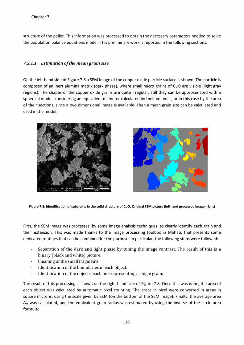
Chapter 7
116
structure of the pellet. This information was processed to obtain the necessary parameters needed to solve
the population balance equations model. This preliminary work is reported in the following sections.
7.5.1.1 Estimation of the mean grain size
On the left hand side of Figure 7.8 a SEM image of the copper oxide particle surface is shown. The particle is
composed of an inert alumina matrix (dark phase), where small micro grains of CuO are visible (light gray
regions). The shapes of the copper oxide grains are quite irregular, still they can be approximated with a
spherical model, considering an equivalent diameter calculated by their volumes, or in this case by the area
of their sections, since a two dimensional image is available. Then a mean grain size can be calculated and
used in the model.
Figure 7.8: Identification of subgrains in the solid structure of CuO. Original SEM picture (left) and processed image (right)
First, the SEM image was processes, by some image analysis techniques, to clearly identify each grain and
their extension. This was made thanks to the image processing toolbox in Matlab, that presents some
dedicated routines that can be combined for the purpose. In particular, the following steps were followed:
- Separation of the dark and light phase by tuning the image contrast. The result of this is a
binary (black and white) picture.
- Cleaning of the small fragments.
- Identification of the boundaries of each object.
- Identification of the objects, each one representing a single grain.
The result of this processing is shown on the right hand side of Figure 7.8. Once this was done, the area of
each object was calculated by automatic pixel counting. The areas in pixel were converted in areas in
square microns, using the scale given by SEM (on the bottom of the SEM image). Finally, the average area
Am was calculated, and the equivalent grain radius was estimated by using the inverse of the circle area
formula:
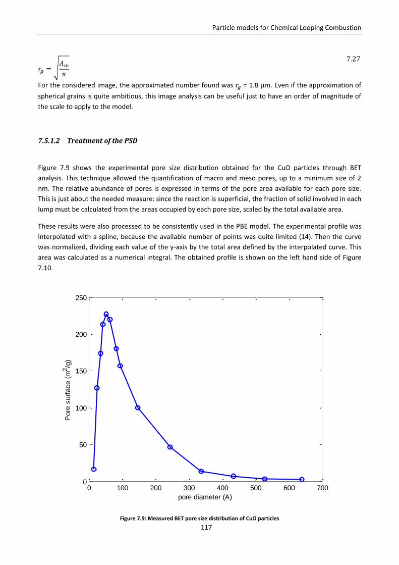
Particle models for Chemical Looping Combustion
117
7.27
For the considered image, the approximated number found was = 1.8 µm. Even if the approximation of
spherical grains is quite ambitious, this image analysis can be useful just to have an order of magnitude of
the scale to apply to the model.
7.5.1.2 Treatment of the PSD
Figure 7.9 shows the experimental pore size distribution obtained for the CuO particles through BET
analysis. This technique allowed the quantification of macro and meso pores, up to a minimum size of 2
nm. The relative abundance of pores is expressed in terms of the pore area available for each pore size.
This is just about the needed measure: since the reaction is superficial, the fraction of solid involved in each
lump must be calculated from the areas occupied by each pore size, scaled by the total available area.
These results were also processed to be consistently used in the PBE model. The experimental profile was
interpolated with a spline, because the available number of points was quite limited (14). Then the curve
was normalized, dividing each value of the y-axis by the total area defined by the interpolated curve. This
area was calculated as a numerical integral. The obtained profile is shown on the left hand side of Figure
7.10.
Figure 7.9: Measured BET pore size distribution of CuO particles
0 100 200 300 400 500 600 7000
50
100
150
200
250
pore diameter (A)
Pore
surf
ace (
m2/g
)
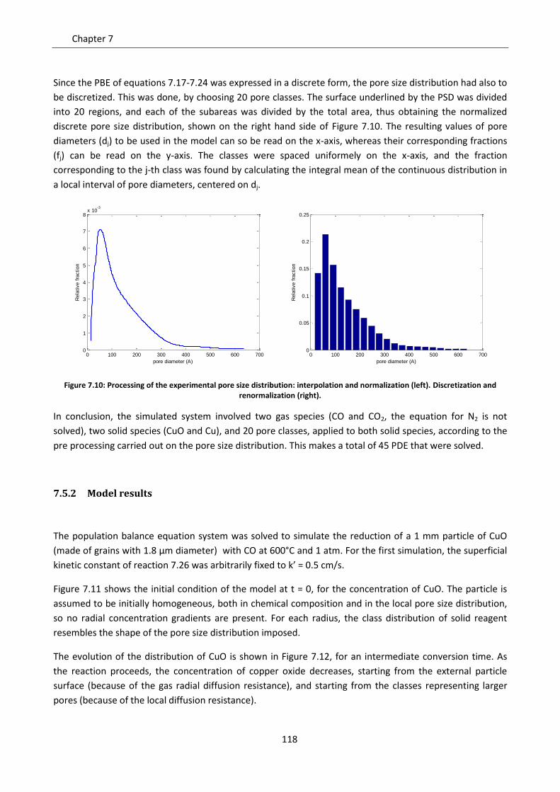
Chapter 7
118
Since the PBE of equations 7.17-7.24 was expressed in a discrete form, the pore size distribution had also to
be discretized. This was done, by choosing 20 pore classes. The surface underlined by the PSD was divided
into 20 regions, and each of the subareas was divided by the total area, thus obtaining the normalized
discrete pore size distribution, shown on the right hand side of Figure 7.10. The resulting values of pore
diameters (dj) to be used in the model can so be read on the x-axis, whereas their corresponding fractions
(fj) can be read on the y-axis. The classes were spaced uniformely on the x-axis, and the fraction
corresponding to the j-th class was found by calculating the integral mean of the continuous distribution in
a local interval of pore diameters, centered on dj.
Figure 7.10: Processing of the experimental pore size distribution: interpolation and normalization (left). Discretization and renormalization (right).
In conclusion, the simulated system involved two gas species (CO and CO2, the equation for N2 is not
solved), two solid species (CuO and Cu), and 20 pore classes, applied to both solid species, according to the
pre processing carried out on the pore size distribution. This makes a total of 45 PDE that were solved.
7.5.2 Model results
The population balance equation system was solved to simulate the reduction of a 1 mm particle of CuO
(made of grains with 1.8 µm diameter) with CO at 600°C and 1 atm. For the first simulation, the superficial
kinetic constant of reaction 7.26 was arbitrarily fixed to k’ = 0.5 cm/s.
Figure 7.11 shows the initial condition of the model at t = 0, for the concentration of CuO. The particle is
assumed to be initially homogeneous, both in chemical composition and in the local pore size distribution,
so no radial concentration gradients are present. For each radius, the class distribution of solid reagent
resembles the shape of the pore size distribution imposed.
The evolution of the distribution of CuO is shown in Figure 7.12, for an intermediate conversion time. As
the reaction proceeds, the concentration of copper oxide decreases, starting from the external particle
surface (because of the gas radial diffusion resistance), and starting from the classes representing larger
pores (because of the local diffusion resistance).
0 100 200 300 400 500 600 7000
1
2
3
4
5
6
7
8x 10
-3
pore diameter (A)
Rela
tive f
raction
0 100 200 300 400 500 600 7000
0.05
0.1
0.15
0.2
0.25
pore diameter (A)
Rela
tive f
raction
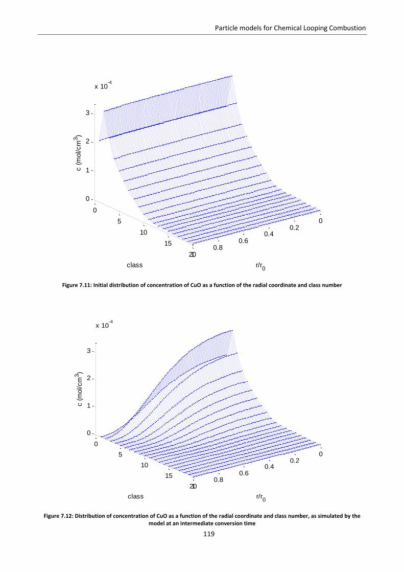
Particle models for Chemical Looping Combustion
119
Figure 7.11: Initial distribution of concentration of CuO as a function of the radial coordinate and class number
Figure 7.12: Distribution of concentration of CuO as a function of the radial coordinate and class number, as simulated by the model at an intermediate conversion time
00.2
0.40.6
0.81
0
5
10
15
20
0
1
2
3
x 10-4
r/r0
class
c (
mol/cm
3)
00.2
0.40.6
0.81
0
5
10
15
20
0
1
2
3
x 10-4
r/r0
class
c (
mol/cm
3)
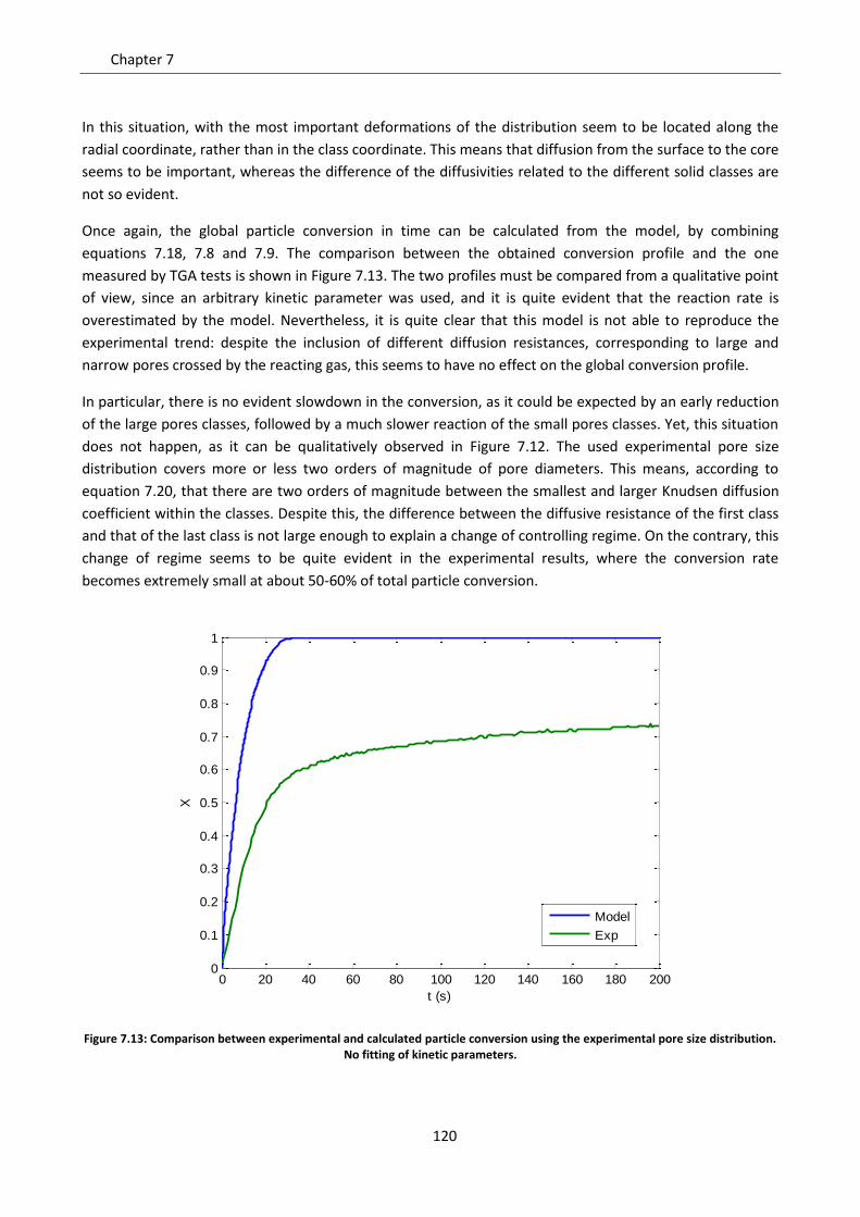
Chapter 7
120
In this situation, with the most important deformations of the distribution seem to be located along the
radial coordinate, rather than in the class coordinate. This means that diffusion from the surface to the core
seems to be important, whereas the difference of the diffusivities related to the different solid classes are
not so evident.
Once again, the global particle conversion in time can be calculated from the model, by combining
equations 7.18, 7.8 and 7.9. The comparison between the obtained conversion profile and the one
measured by TGA tests is shown in Figure 7.13. The two profiles must be compared from a qualitative point
of view, since an arbitrary kinetic parameter was used, and it is quite evident that the reaction rate is
overestimated by the model. Nevertheless, it is quite clear that this model is not able to reproduce the
experimental trend: despite the inclusion of different diffusion resistances, corresponding to large and
narrow pores crossed by the reacting gas, this seems to have no effect on the global conversion profile.
In particular, there is no evident slowdown in the conversion, as it could be expected by an early reduction
of the large pores classes, followed by a much slower reaction of the small pores classes. Yet, this situation
does not happen, as it can be qualitatively observed in Figure 7.12. The used experimental pore size
distribution covers more or less two orders of magnitude of pore diameters. This means, according to
equation 7.20, that there are two orders of magnitude between the smallest and larger Knudsen diffusion
coefficient within the classes. Despite this, the difference between the diffusive resistance of the first class
and that of the last class is not large enough to explain a change of controlling regime. On the contrary, this
change of regime seems to be quite evident in the experimental results, where the conversion rate
becomes extremely small at about 50-60% of total particle conversion.
Figure 7.13: Comparison between experimental and calculated particle conversion using the experimental pore size distribution. No fitting of kinetic parameters.
0 20 40 60 80 100 120 140 160 180 2000
0.1
0.2
0.3
0.4
0.5
0.6
0.7
0.8
0.9
1
t (s)
X
Model
Exp
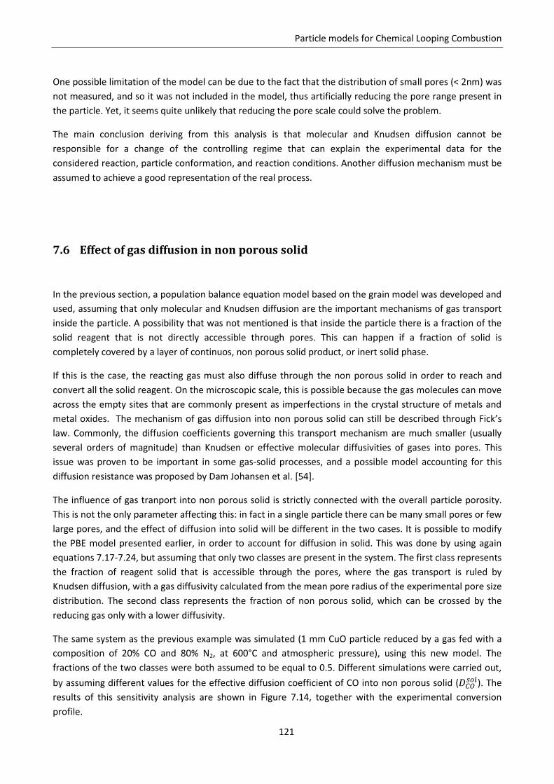
Particle models for Chemical Looping Combustion
121
One possible limitation of the model can be due to the fact that the distribution of small pores (< 2nm) was
not measured, and so it was not included in the model, thus artificially reducing the pore range present in
the particle. Yet, it seems quite unlikely that reducing the pore scale could solve the problem.
The main conclusion deriving from this analysis is that molecular and Knudsen diffusion cannot be
responsible for a change of the controlling regime that can explain the experimental data for the
considered reaction, particle conformation, and reaction conditions. Another diffusion mechanism must be
assumed to achieve a good representation of the real process.
7.6 Effect of gas diffusion in non porous solid
In the previous section, a population balance equation model based on the grain model was developed and
used, assuming that only molecular and Knudsen diffusion are the important mechanisms of gas transport
inside the particle. A possibility that was not mentioned is that inside the particle there is a fraction of the
solid reagent that is not directly accessible through pores. This can happen if a fraction of solid is
completely covered by a layer of continuos, non porous solid product, or inert solid phase.
If this is the case, the reacting gas must also diffuse through the non porous solid in order to reach and
convert all the solid reagent. On the microscopic scale, this is possible because the gas molecules can move
across the empty sites that are commonly present as imperfections in the crystal structure of metals and
metal oxides. The mechanism of gas diffusion into non porous solid can still be described through Fick’s
law. Commonly, the diffusion coefficients governing this transport mechanism are much smaller (usually
several orders of magnitude) than Knudsen or effective molecular diffusivities of gases into pores. This
issue was proven to be important in some gas-solid processes, and a possible model accounting for this
diffusion resistance was proposed by Dam Johansen et al. [54].
The influence of gas tranport into non porous solid is strictly connected with the overall particle porosity.
This is not the only parameter affecting this: in fact in a single particle there can be many small pores or few
large pores, and the effect of diffusion into solid will be different in the two cases. It is possible to modify
the PBE model presented earlier, in order to account for diffusion in solid. This was done by using again
equations 7.17-7.24, but assuming that only two classes are present in the system. The first class represents
the fraction of reagent solid that is accessible through the pores, where the gas transport is ruled by
Knudsen diffusion, with a gas diffusivity calculated from the mean pore radius of the experimental pore size
distribution. The second class represents the fraction of non porous solid, which can be crossed by the
reducing gas only with a lower diffusivity.
The same system as the previous example was simulated (1 mm CuO particle reduced by a gas fed with a
composition of 20% CO and 80% N2, at 600°C and atmospheric pressure), using this new model. The
fractions of the two classes were both assumed to be equal to 0.5. Different simulations were carried out,
by assuming different values for the effective diffusion coefficient of CO into non porous solid ( ). The
results of this sensitivity analysis are shown in Figure 7.14, together with the experimental conversion
profile.
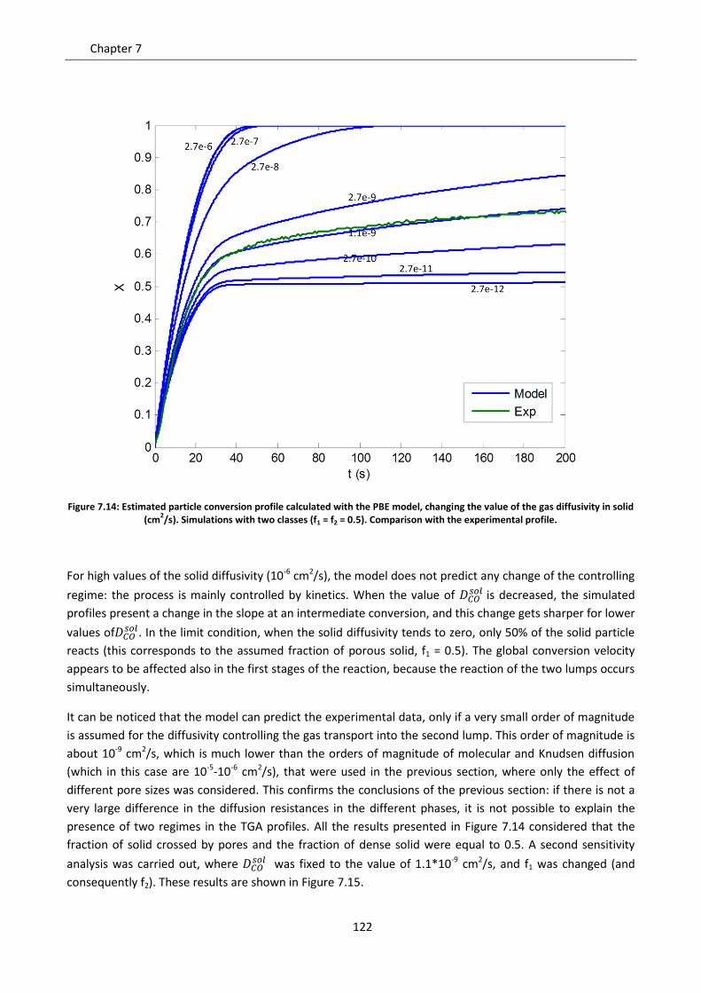
Chapter 7
122
Figure 7.14: Estimated particle conversion profile calculated with the PBE model, changing the value of the gas diffusivity in solid (cm
2/s). Simulations with two classes (f1 = f2 = 0.5). Comparison with the experimental profile.
For high values of the solid diffusivity (10-6 cm2/s), the model does not predict any change of the controlling
regime: the process is mainly controlled by kinetics. When the value of
is decreased, the simulated
profiles present a change in the slope at an intermediate conversion, and this change gets sharper for lower
values of . In the limit condition, when the solid diffusivity tends to zero, only 50% of the solid particle
reacts (this corresponds to the assumed fraction of porous solid, f1 = 0.5). The global conversion velocity
appears to be affected also in the first stages of the reaction, because the reaction of the two lumps occurs
simultaneously.
It can be noticed that the model can predict the experimental data, only if a very small order of magnitude
is assumed for the diffusivity controlling the gas transport into the second lump. This order of magnitude is
about 10-9 cm2/s, which is much lower than the orders of magnitude of molecular and Knudsen diffusion
(which in this case are 10-5-10-6 cm2/s), that were used in the previous section, where only the effect of
different pore sizes was considered. This confirms the conclusions of the previous section: if there is not a
very large difference in the diffusion resistances in the different phases, it is not possible to explain the
presence of two regimes in the TGA profiles. All the results presented in Figure 7.14 considered that the
fraction of solid crossed by pores and the fraction of dense solid were equal to 0.5. A second sensitivity
analysis was carried out, where
was fixed to the value of 1.1*10-9 cm2/s, and f1 was changed (and
consequently f2). These results are shown in Figure 7.15.
Particle models for Chemical Looping Combustion
123
Figure 7.15: Estimated particle conversion profile calculated with the PBE model, assuming the value of the gas diffusivity in solid equal to 1.1*10
-9 cm
2/s, for different values of fractions of porous solid f1. Comparison with the experimental profile.
The different simulations show that the relative fractions of solid and dense material can have an important
influence on the model results. The velocity of conversion in the second stage (identified by the slope of the
profiles at long times) does not change, in fact this is identified by the value of which is always the
same. What is different is the conversion at which the simulated profile bends, which corresponds to the
point when the fraction of porous material (f1) has more or less completely converted, and only the dense
solid reagent (f2) remains. Also, the slope of the first stage can change, because of the presence of two
combined resistances.
A final sensitivity test was made. This time, was again fixed to the optimum value of 1.1*10-9 cm2/s,
and the fractions of porous and dense material were also fixed (f1 = f2 = 0.5). Different simulations were
carried out, changing the kinetic constant k’ of the model. The results are shown in Figure 7.16. The curves
are parametric to a Thiele modulus , calculated as follows:
7.28
In this formulation, is the Knudsen diffusion coefficient of CO into the porous fraction, calculated from
the average pore size and used to describe the gas reaction rate into the equation for the first class. It can
be noticed that, for all the simulations, is well below unity, which means that for all the cases the early
conversion step, corresponding to the reaction of the porous fraction of the particle, is controlled by
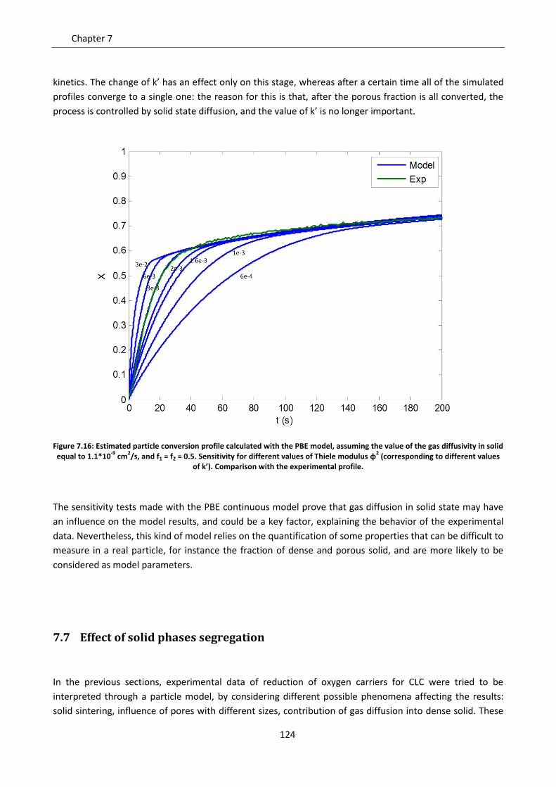
Chapter 7
124
kinetics. The change of k’ has an effect only on this stage, whereas after a certain time all of the simulated
profiles converge to a single one: the reason for this is that, after the porous fraction is all converted, the
process is controlled by solid state diffusion, and the value of k’ is no longer important.
Figure 7.16: Estimated particle conversion profile calculated with the PBE model, assuming the value of the gas diffusivity in solid equal to 1.1*10
-9 cm
2/s, and f1 = f2 = 0.5. Sensitivity for different values of Thiele modulus φ
2 (corresponding to different values
of k’). Comparison with the experimental profile.
The sensitivity tests made with the PBE continuous model prove that gas diffusion in solid state may have
an influence on the model results, and could be a key factor, explaining the behavior of the experimental
data. Nevertheless, this kind of model relies on the quantification of some properties that can be difficult to
measure in a real particle, for instance the fraction of dense and porous solid, and are more likely to be
considered as model parameters.
7.7 Effect of solid phases segregation
In the previous sections, experimental data of reduction of oxygen carriers for CLC were tried to be
interpreted through a particle model, by considering different possible phenomena affecting the results:
solid sintering, influence of pores with different sizes, contribution of gas diffusion into dense solid. These
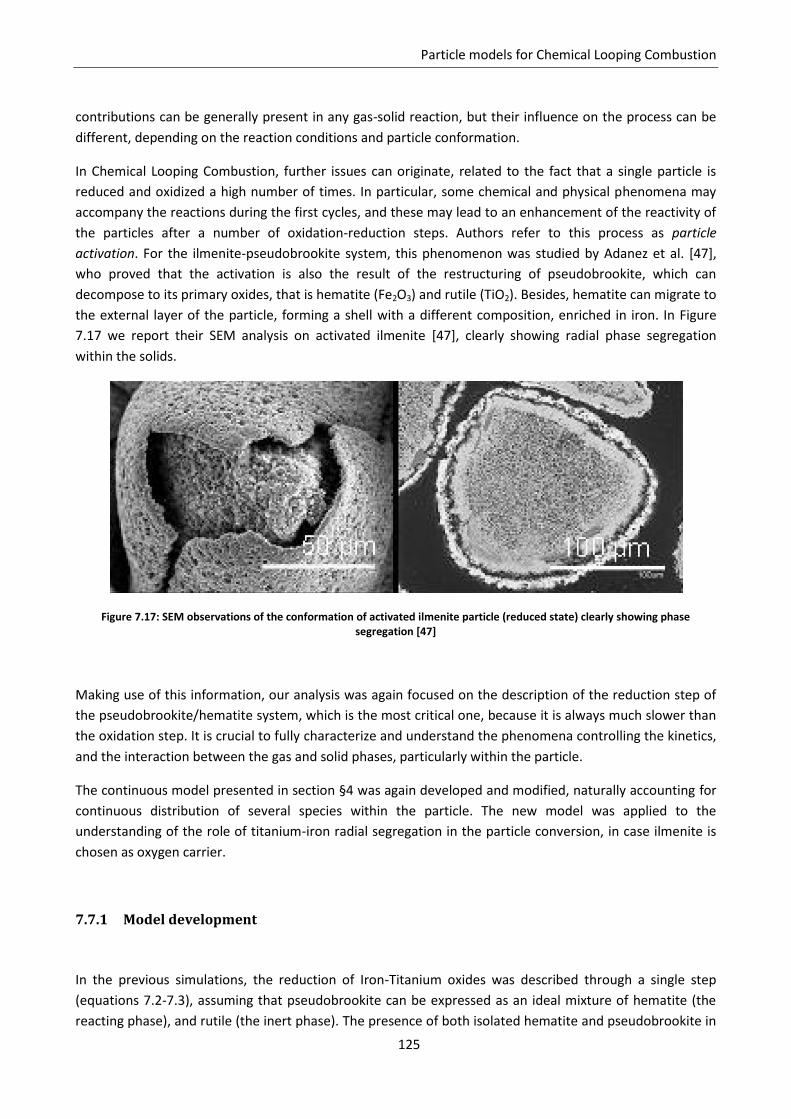
Particle models for Chemical Looping Combustion
125
contributions can be generally present in any gas-solid reaction, but their influence on the process can be
different, depending on the reaction conditions and particle conformation.
In Chemical Looping Combustion, further issues can originate, related to the fact that a single particle is
reduced and oxidized a high number of times. In particular, some chemical and physical phenomena may
accompany the reactions during the first cycles, and these may lead to an enhancement of the reactivity of
the particles after a number of oxidation-reduction steps. Authors refer to this process as particle
activation. For the ilmenite-pseudobrookite system, this phenomenon was studied by Adanez et al. [47],
who proved that the activation is also the result of the restructuring of pseudobrookite, which can
decompose to its primary oxides, that is hematite (Fe2O3) and rutile (TiO2). Besides, hematite can migrate to
the external layer of the particle, forming a shell with a different composition, enriched in iron. In Figure
7.17 we report their SEM analysis on activated ilmenite [47], clearly showing radial phase segregation
within the solids.
Figure 7.17: SEM observations of the conformation of activated ilmenite particle (reduced state) clearly showing phase segregation [47]
Making use of this information, our analysis was again focused on the description of the reduction step of
the pseudobrookite/hematite system, which is the most critical one, because it is always much slower than
the oxidation step. It is crucial to fully characterize and understand the phenomena controlling the kinetics,
and the interaction between the gas and solid phases, particularly within the particle.
The continuous model presented in section §4 was again developed and modified, naturally accounting for
continuous distribution of several species within the particle. The new model was applied to the
understanding of the role of titanium-iron radial segregation in the particle conversion, in case ilmenite is
chosen as oxygen carrier.
7.7.1 Model development
In the previous simulations, the reduction of Iron-Titanium oxides was described through a single step
(equations 7.2-7.3), assuming that pseudobrookite can be expressed as an ideal mixture of hematite (the
reacting phase), and rutile (the inert phase). The presence of both isolated hematite and pseudobrookite in
Chapter 7
126
the activated particles, on the contrary, can suggest that both phases can react in parallel, possibly with a
different kinetic rate.
A new reaction scheme was used, including both the reduction of hematite to wustite and the reduction of
pseudobrookite to ilmenite. If hydrogen is the fuel, this is:
7.29
7.30
Analogously, for the reduction with CO:
7.31
7.32
More elaborated reaction systems could account for the presence of ulvospinel (Fe2TiO4), a reduced species
which is thermodynamically unstable [55]. Interestingly, ilmenite and hematite can be perfectly miscible at
high temperature, but not at lower ones. Given that the process cycles over the temperature, restructuring
of the particle should be expected, leading to solid phase segregation. Note that two reactions sharing the
same reagents are incompatible with the existence of two sharp reactions fronts within the particles, as
assumed by the shrinking core model, where reactions need to be much faster than diffusion. The
outermost interface is expected to consume all the reagent, i.e. CO or H2, preventing its transport to the
inner interface, to feed the other reaction.
To describe the evolution of the reactive particle with a continuous model, the conservation balances were
solved assuming spherical geometry of the particles. Again, the continuous model in the form of equations
4.37-4.41 was used, considering no change of particle size. The Stefan-Maxwell model was used to describe
the diffusive fluxes of the gas species (equations 5.43-5.47), including Knudsen diffusion (equation 5.93),
whereas the evolution of local porosity was expressed through equation 4.45. The boundary and initial
conditions used were in the form of equations 4.47, 4.48 and 4.50.
The reaction rates can be considered to be first order in the concentration of the gas reactant (H2 or CO),
and non linearly on the solid conversions Xi, with i=H(ematite) or i=P(seudobrookite), as follows:
7.33
7.34
7.35
7.36
In equations 7.33-7.36, the conversions of the single solid species are defined as follows:
Particle models for Chemical Looping Combustion
127
7.37
7.38
The function f(X) was expressed through the grain model, according to equation 4.71.
A possible variation of the form of the reaction rates was also considered: in alternative to equations (7.33-
7.36), the reaction rates can be also expressed by means of a Langmuir-type equation, which can take into
account possible resistances due to a finite adsorption rate of the reagent gas:
7.39
7.40
7.41
7.42
In this formulation, four additional parameters K1, K2, K3, K4 must be provided, possibly depending on
temperature. The Langmuir approach can be more suitable if the reaction dependency on the
concentration of the reactant gas is apparently less than first order.
In any case, kinetic constants, k1, k2, k3, k4, must be specified as functions of temperature, by means of the
Arrhenius law (eq. 4.54).
The model was solved using a finite difference method to discretize the space derivatives [56]. A centered
differences scheme was used for the diffusion term, while first order upwind was chosen for the convective
terms. The theta method was used to handle the time derivatives. In particular, Cranck-Nicholson scheme
[57] was chosen (θ = ½). The problem was finally solved by linearizing the non linear (convection and
reaction) terms with a Newton scheme, and thus solving iteratively the linear system obtained by
introducing a Jacobian matrix that was calculated analytically.
From the model results, again the global particle conversion can be calculated through equations 7.8-7.9.
7.7.2 Model predictions and sensitivity to non uniform initial conditions
Before attempting any comparison of experimental data and model predictions, and subsequent parameter
estimation, an investigation on the significance of the initial solids composition and the competition of the
two reactions steps has been carried out.
Chapter 7
128
Typically, simulations assume a uniform initial composition of the particles, i.e. constant radial
concentration profiles for all the solid species in the pellet. If solid phase segregation is present at the
beginning of the reaction, as shown in Figure 7.17 because of activation, the initial conditions must be
modified accordingly. In addition, the solid migration phenomenon should be considered in a time
dependent simulation, but this is quite slow if compared to the chemical reaction, and it has eventually no
effect in activated particles. For this reason it can be neglected while simulating a single reduction step, but
it might be important to include it while solving a high number of cycles, particularly during the first cycles
that involve non activated solids. In this present work, the reaction was simulated for particles where
migration has already occurred, and the oxidized phases are already segregated forming a core-shell
structure. This mathematically is translated into non uniform initial solid radial concentration profiles.
The reaction of hematite and pseudobrookite can occur in series or in parallel. They take place in series if
one of the two solid reagents is segregated in the outer region of the particle and the other one in the core,
and also the reaction evolves like a shrinking core model. In this case, the reacting gas will first meet the
outer solid phase, and eventually the inner phase, but only when the first one is completely oxidized. A
shrinking core behavior is possible only if diffusion is controlling over the reaction rates, so in this case a
different reactivity of Fe2O3 and Fe2TiO5 should not determine any change in the conversion rate. Yet, this
could be the consequence of different effective diffusivities of the reagent gas in the two layers (for
example if the porosities are very different from each others). A diffusive regime is usually possible for large
particles, or particles with a quite dense solid matrix.
On the contrary, the two reaction steps take place in parallel if there is no phase segregation, or if there is
segregation but the process is controlled by kinetics: in this case the reacting gas is always present
throughout the particle, so both Fe2O3 and Fe2TiO5 react simultaneously even if one is in the core and the
other in the shell of the particle. Nevertheless, if one of the two steps is much faster than the other, there
will be a time when the fast reacting solid is completely reduced, while the second one is not. This could
also cause a shift in the global conversion profiles.
In order to reproduce the initial core shell structure, and identify the initial composition profiles for the
solid species inside the particle, some degrees of freedom must be fixed. They are:
- The radial position of the interface dividing the core and the shell.
- The relative composition of the core and the shell.
In the chemistry chosen here, three solid species are present before the reduction of the particles, namely
hematite (Fe2O3), pseudobrookite (Fe2TiO5), and rutile (TiO2). This makes a total of seven variables to set
just to describe the initial conditions: they are the concentration of Fe2O3, Fe2TiO5 and TiO2 in the core and
in the shell, and the radial position of the core-shell interface.
Some constraints can also be set. First, if the global fraction of iron and titanium of the particle is known, it
will be:
7.43
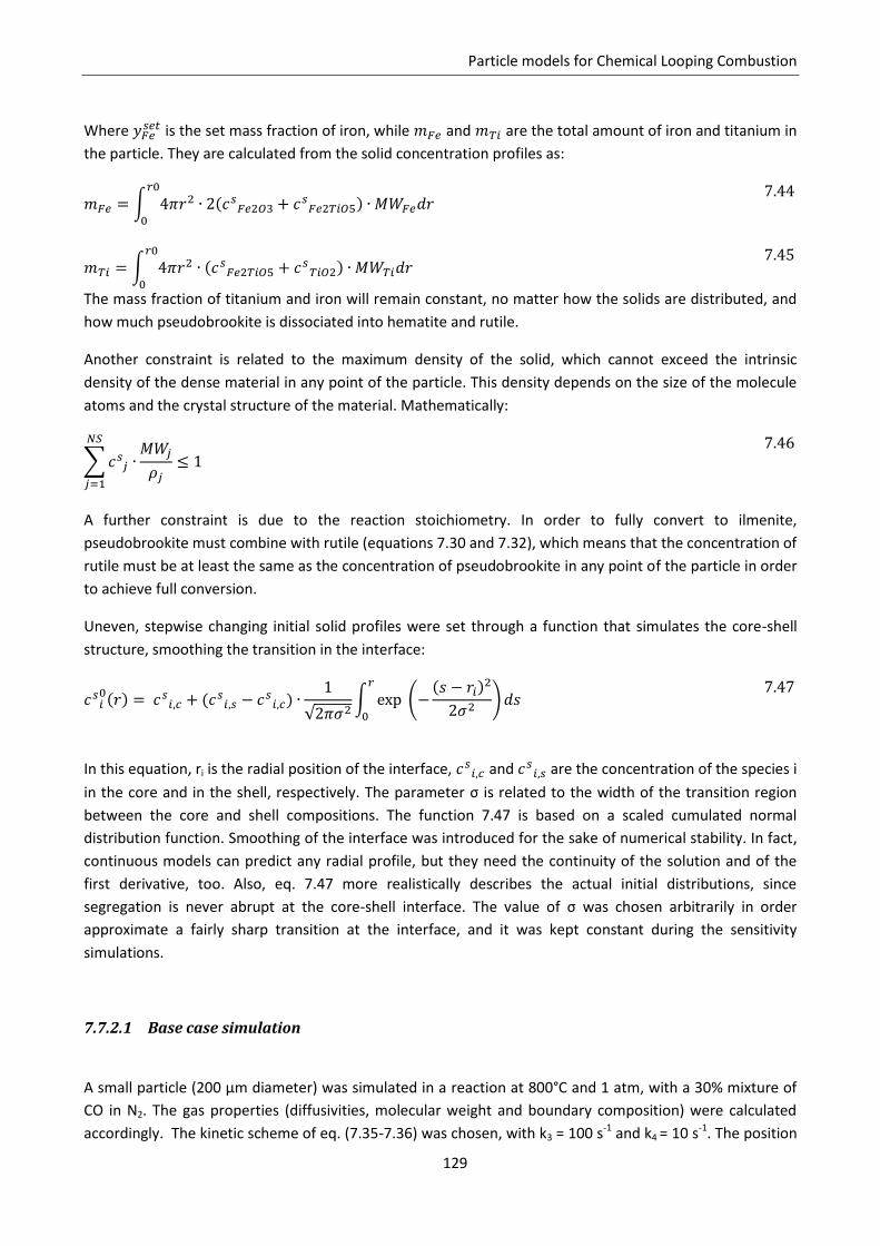
Particle models for Chemical Looping Combustion
129
Where is the set mass fraction of iron, while and are the total amount of iron and titanium in
the particle. They are calculated from the solid concentration profiles as:
7.44
7.45
The mass fraction of titanium and iron will remain constant, no matter how the solids are distributed, and
how much pseudobrookite is dissociated into hematite and rutile.
Another constraint is related to the maximum density of the solid, which cannot exceed the intrinsic
density of the dense material in any point of the particle. This density depends on the size of the molecule
atoms and the crystal structure of the material. Mathematically:
7.46
A further constraint is due to the reaction stoichiometry. In order to fully convert to ilmenite,
pseudobrookite must combine with rutile (equations 7.30 and 7.32), which means that the concentration of
rutile must be at least the same as the concentration of pseudobrookite in any point of the particle in order
to achieve full conversion.
Uneven, stepwise changing initial solid profiles were set through a function that simulates the core-shell
structure, smoothing the transition in the interface:
7.47
In this equation, ri is the radial position of the interface, and
are the concentration of the species i
in the core and in the shell, respectively. The parameter σ is related to the width of the transition region
between the core and shell compositions. The function 7.47 is based on a scaled cumulated normal
distribution function. Smoothing of the interface was introduced for the sake of numerical stability. In fact,
continuous models can predict any radial profile, but they need the continuity of the solution and of the
first derivative, too. Also, eq. 7.47 more realistically describes the actual initial distributions, since
segregation is never abrupt at the core-shell interface. The value of σ was chosen arbitrarily in order
approximate a fairly sharp transition at the interface, and it was kept constant during the sensitivity
simulations.
7.7.2.1 Base case simulation
A small particle (200 μm diameter) was simulated in a reaction at 800°C and 1 atm, with a 30% mixture of
CO in N2. The gas properties (diffusivities, molecular weight and boundary composition) were calculated
accordingly. The kinetic scheme of eq. (7.35-7.36) was chosen, with k3 = 100 s-1 and k4 = 10 s-1. The position
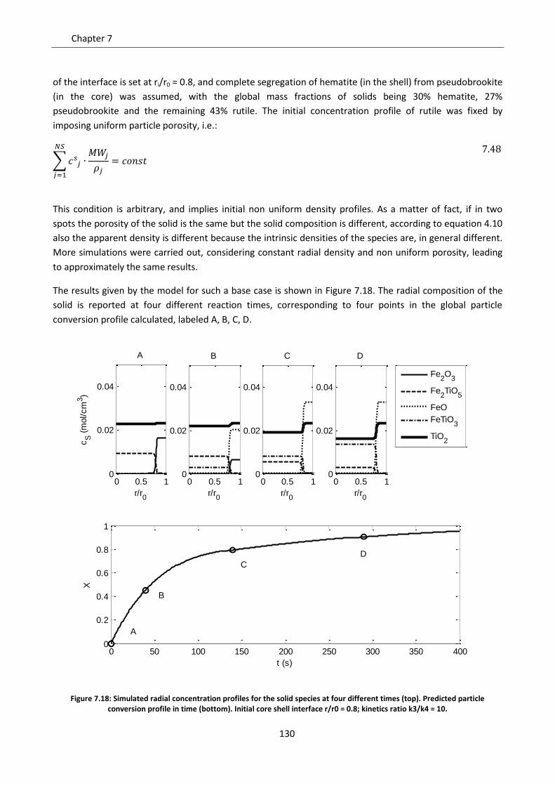
Chapter 7
130
of the interface is set at ri/r0 = 0.8, and complete segregation of hematite (in the shell) from pseudobrookite
(in the core) was assumed, with the global mass fractions of solids being 30% hematite, 27%
pseudobrookite and the remaining 43% rutile. The initial concentration profile of rutile was fixed by
imposing uniform particle porosity, i.e.:
7.48
This condition is arbitrary, and implies initial non uniform density profiles. As a matter of fact, if in two
spots the porosity of the solid is the same but the solid composition is different, according to equation 4.10
also the apparent density is different because the intrinsic densities of the species are, in general different.
More simulations were carried out, considering constant radial density and non uniform porosity, leading
to approximately the same results.
The results given by the model for such a base case is shown in Figure 7.18. The radial composition of the
solid is reported at four different reaction times, corresponding to four points in the global particle
conversion profile calculated, labeled A, B, C, D.
Figure 7.18: Simulated radial concentration profiles for the solid species at four different times (top). Predicted particle conversion profile in time (bottom). Initial core shell interface r/r0 = 0.8; kinetics ratio k3/k4 = 10.
0 0.5 10
0.02
0.04
r/r0
cS (
mol/cm
3)
A
0 0.5 10
0.02
0.04
r/r0
B
0 0.5 10
0.02
0.04
r/r0
C
0 0.5 10
0.02
0.04
r/r0
D
Fe
2O
3
Fe2TiO
5
FeO
FeTiO3
TiO2
0 50 100 150 200 250 300 350 4000
0.2
0.4
0.6
0.8
1
t (s)
X
B
C
D
A
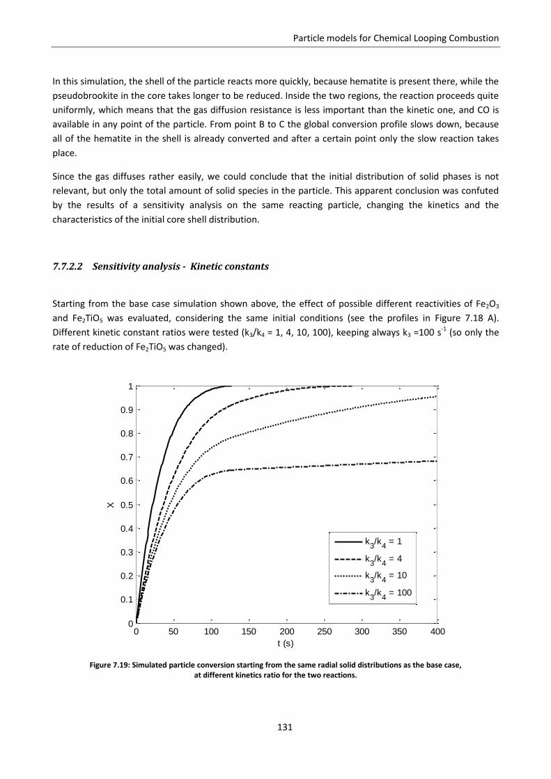
Particle models for Chemical Looping Combustion
131
In this simulation, the shell of the particle reacts more quickly, because hematite is present there, while the
pseudobrookite in the core takes longer to be reduced. Inside the two regions, the reaction proceeds quite
uniformly, which means that the gas diffusion resistance is less important than the kinetic one, and CO is
available in any point of the particle. From point B to C the global conversion profile slows down, because
all of the hematite in the shell is already converted and after a certain point only the slow reaction takes
place.
Since the gas diffuses rather easily, we could conclude that the initial distribution of solid phases is not
relevant, but only the total amount of solid species in the particle. This apparent conclusion was confuted
by the results of a sensitivity analysis on the same reacting particle, changing the kinetics and the
characteristics of the initial core shell distribution.
7.7.2.2 Sensitivity analysis - Kinetic constants
Starting from the base case simulation shown above, the effect of possible different reactivities of Fe2O3
and Fe2TiO5 was evaluated, considering the same initial conditions (see the profiles in Figure 7.18 A).
Different kinetic constant ratios were tested (k3/k4 = 1, 4, 10, 100), keeping always k3 =100 s-1 (so only the
rate of reduction of Fe2TiO5 was changed).
Figure 7.19: Simulated particle conversion starting from the same radial solid distributions as the base case, at different kinetics ratio for the two reactions.
0 50 100 150 200 250 300 350 4000
0.1
0.2
0.3
0.4
0.5
0.6
0.7
0.8
0.9
1
t (s)
X
k3/k
4 = 1
k3/k
4 = 4
k3/k
4 = 10
k3/k
4 = 100
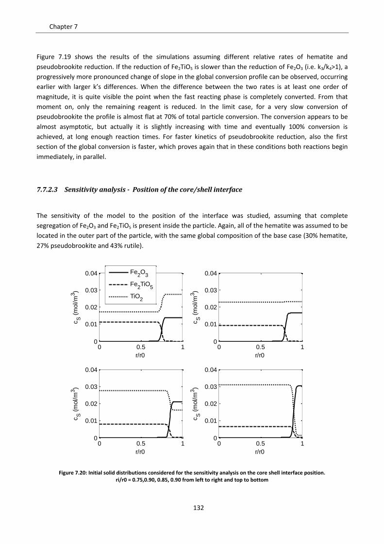
Chapter 7
132
Figure 7.19 shows the results of the simulations assuming different relative rates of hematite and
pseudobrookite reduction. If the reduction of Fe2TiO5 is slower than the reduction of Fe2O3 (i.e. k3/k4>1), a
progressively more pronounced change of slope in the global conversion profile can be observed, occurring
earlier with larger k’s differences. When the difference between the two rates is at least one order of
magnitude, it is quite visible the point when the fast reacting phase is completely converted. From that
moment on, only the remaining reagent is reduced. In the limit case, for a very slow conversion of
pseudobrookite the profile is almost flat at 70% of total particle conversion. The conversion appears to be
almost asymptotic, but actually it is slightly increasing with time and eventually 100% conversion is
achieved, at long enough reaction times. For faster kinetics of pseudobrookite reduction, also the first
section of the global conversion is faster, which proves again that in these conditions both reactions begin
immediately, in parallel.
7.7.2.3 Sensitivity analysis - Position of the core/shell interface
The sensitivity of the model to the position of the interface was studied, assuming that complete
segregation of Fe2O3 and Fe2TiO5 is present inside the particle. Again, all of the hematite was assumed to be
located in the outer part of the particle, with the same global composition of the base case (30% hematite,
27% pseudobrookite and 43% rutile).
Figure 7.20: Initial solid distributions considered for the sensitivity analysis on the core shell interface position. ri/r0 = 0.75,0.90, 0.85, 0.90 from left to right and top to bottom
0 0.5 10
0.01
0.02
0.03
0.04
r/r0
cS (
mol/m
3)
0 0.5 10
0.01
0.02
0.03
0.04
r/r0
cS (
mol/m
3)
0 0.5 10
0.01
0.02
0.03
0.04
r/r0
cS (
mol/m
3)
0 0.5 10
0.01
0.02
0.03
0.04
r/r0
cS (
mol/m
3)
Fe2O
3
Fe2TiO
5
TiO2
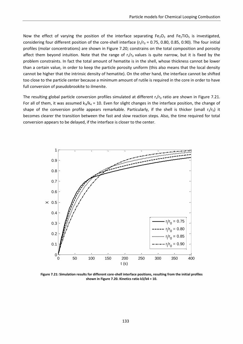
Particle models for Chemical Looping Combustion
133
Now the effect of varying the position of the interface separating Fe2O3 and Fe2TiO5 is investigated,
considering four different position of the core-shell interface (ri/r0 = 0.75, 0.80, 0.85, 0.90). The four initial
profiles (molar concentrations) are shown in Figure 7.20; constrains on the total composition and porosity
affect them beyond intuition. Note that the range of ri/r0 values is quite narrow, but it is fixed by the
problem constraints. In fact the total amount of hematite is in the shell, whose thickness cannot be lower
than a certain value, in order to keep the particle porosity uniform (this also means that the local density
cannot be higher that the intrinsic density of hematite). On the other hand, the interface cannot be shifted
too close to the particle center because a minimum amount of rutile is required in the core in order to have
full conversion of pseudobrookite to ilmenite.
The resulting global particle conversion profiles simulated at different ri/r0 ratio are shown in Figure 7.21.
For all of them, it was assumed k3/k4 = 10. Even for slight changes in the interface position, the change of
shape of the conversion profile appears remarkable. Particularly, if the shell is thicker (small ri/r0) it
becomes clearer the transition between the fast and slow reaction steps. Also, the time required for total
conversion appears to be delayed, if the interface is closer to the center.
Figure 7.21: Simulation results for different core-shell interface positions, resulting from the initial profiles shown in Figure 7.20. Kinetics ratio k3/k4 = 10.
0 50 100 150 200 250 300 350 4000
0.1
0.2
0.3
0.4
0.5
0.6
0.7
0.8
0.9
1
t (s)
X
ri/r
0 = 0.75
ri/r
0 = 0.80
ri/r
0 = 0.85
ri/r
0 = 0.90
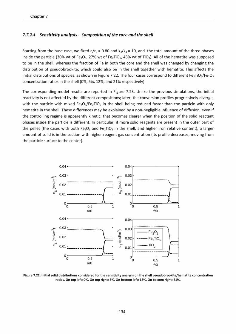
Chapter 7
134
7.7.2.4 Sensitivity analysis - Composition of the core and the shell
Starting from the base case, we fixed ri/r0 = 0.80 and k3/k4 = 10, and the total amount of the three phases
inside the particle (30% wt of Fe2O3, 27% wt of Fe2TiO5, 43% wt of TiO2). All of the hematite was supposed
to be in the shell, whereas the fraction of Fe in both the core and the shell was changed by changing the
distribution of pseudobrookite, which could also be in the shell together with hematite. This affects the
initial distributions of species, as shown in Figure 7.22. The four cases correspond to different Fe2TiO5/Fe2O3
concentration ratios in the shell (0%, 5%, 12%, and 21% respectively).
The corresponding model results are reported in Figure 7.23. Unlike the previous simulations, the initial
reactivity is not affected by the different compositions; later, the conversion profiles progressively diverge,
with the particle with mixed Fe2O3/Fe2TiO5 in the shell being reduced faster than the particle with only
hematite in the shell. These differences may be explained by a non-negligible influence of diffusion, even if
the controlling regime is apparently kinetic; that becomes clearer when the position of the solid reactant
phases inside the particle is different. In particular, if more solid reagents are present in the outer part of
the pellet (the cases with both Fe2O3 and Fe2TiO5 in the shell, and higher iron relative content), a larger
amount of solid is in the section with higher reagent gas concentration (its profile decreases, moving from
the particle surface to the center).
Figure 7.22: Initial solid distributions considered for the sensitivity analysis on the shell pseudobrookite/hematite concentration ratios. On top left: 0%. On top right: 5%. On bottom left: 12%. On bottom right: 21%.
0 0.5 10
0.01
0.02
0.03
0.04
r/r0
cS (
mol/m
3)
0 0.5 10
0.01
0.02
0.03
0.04
r/r0
cS (
mol/m
3)
0 0.5 10
0.01
0.02
0.03
0.04
r/r0
cS (
mol/m
3)
0 0.5 10
0.01
0.02
0.03
0.04
r/r0
cS (
mol/m
3)
Fe2O
3
Fe2TiO
5
TiO2
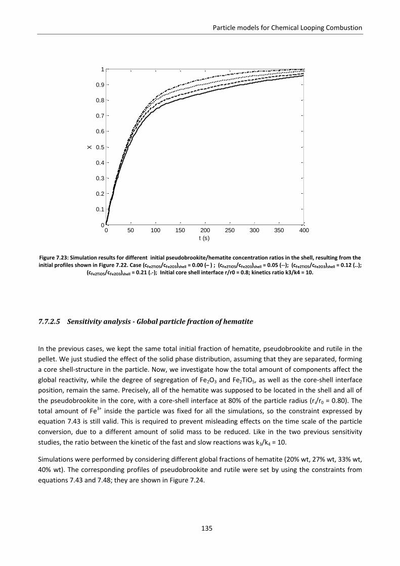
Particle models for Chemical Looping Combustion
135
Figure 7.23: Simulation results for different initial pseudobrookite/hematite concentration ratios in the shell, resulting from the initial profiles shown in Figure 7.22. Case (cFe2TiO5/cFe2O3)shell = 0.00 ( ) ; (cFe2TiO5/cFe2O3)shell = 0.05 (--); (cFe2TiO5/cFe2O3)shell = 0.12 (..);
(cFe2TiO5/cFe2O3)shell = 0.21 (.-); Initial core shell interface r/r0 = 0.8; kinetics ratio k3/k4 = 10.
7.7.2.5 Sensitivity analysis - Global particle fraction of hematite
In the previous cases, we kept the same total initial fraction of hematite, pseudobrookite and rutile in the
pellet. We just studied the effect of the solid phase distribution, assuming that they are separated, forming
a core shell-structure in the particle. Now, we investigate how the total amount of components affect the
global reactivity, while the degree of segregation of Fe2O3 and Fe2TiO5, as well as the core-shell interface
position, remain the same. Precisely, all of the hematite was supposed to be located in the shell and all of
the pseudobrookite in the core, with a core-shell interface at 80% of the particle radius (ri/r0 = 0.80). The
total amount of Fe3+ inside the particle was fixed for all the simulations, so the constraint expressed by
equation 7.43 is still valid. This is required to prevent misleading effects on the time scale of the particle
conversion, due to a different amount of solid mass to be reduced. Like in the two previous sensitivity
studies, the ratio between the kinetic of the fast and slow reactions was k3/k4 = 10.
Simulations were performed by considering different global fractions of hematite (20% wt, 27% wt, 33% wt,
40% wt). The corresponding profiles of pseudobrookite and rutile were set by using the constraints from
equations 7.43 and 7.48; they are shown in Figure 7.24.
0 50 100 150 200 250 300 350 4000
0.1
0.2
0.3
0.4
0.5
0.6
0.7
0.8
0.9
1
t (s)
X
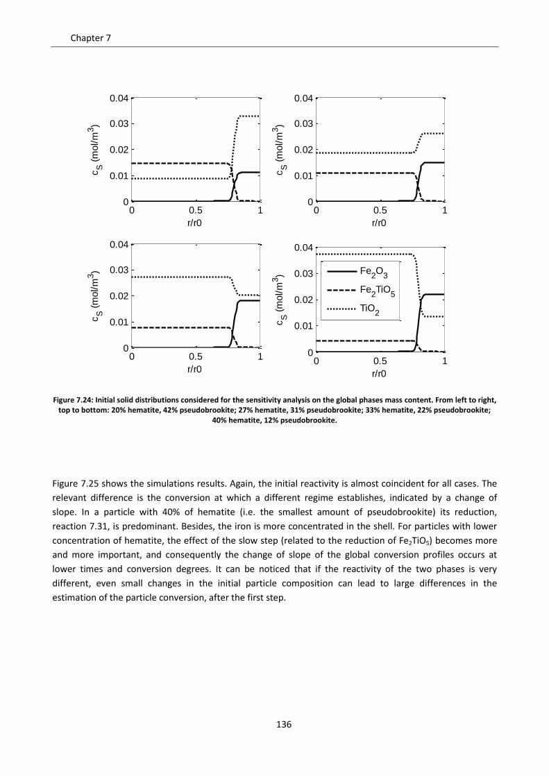
Chapter 7
136
Figure 7.24: Initial solid distributions considered for the sensitivity analysis on the global phases mass content. From left to right, top to bottom: 20% hematite, 42% pseudobrookite; 27% hematite, 31% pseudobrookite; 33% hematite, 22% pseudobrookite;
40% hematite, 12% pseudobrookite.
Figure 7.25 shows the simulations results. Again, the initial reactivity is almost coincident for all cases. The
relevant difference is the conversion at which a different regime establishes, indicated by a change of
slope. In a particle with 40% of hematite (i.e. the smallest amount of pseudobrookite) its reduction,
reaction 7.31, is predominant. Besides, the iron is more concentrated in the shell. For particles with lower
concentration of hematite, the effect of the slow step (related to the reduction of Fe2TiO5) becomes more
and more important, and consequently the change of slope of the global conversion profiles occurs at
lower times and conversion degrees. It can be noticed that if the reactivity of the two phases is very
different, even small changes in the initial particle composition can lead to large differences in the
estimation of the particle conversion, after the first step.
0 0.5 10
0.01
0.02
0.03
0.04
r/r0
cS (
mol/m
3)
0 0.5 10
0.01
0.02
0.03
0.04
r/r0
cS (
mol/m
3)
0 0.5 10
0.01
0.02
0.03
0.04
r/r0
cS (
mol/m
3)
0 0.5 10
0.01
0.02
0.03
0.04
r/r0
cS (
mol/m
3)
Fe2O
3
Fe2TiO
5
TiO2
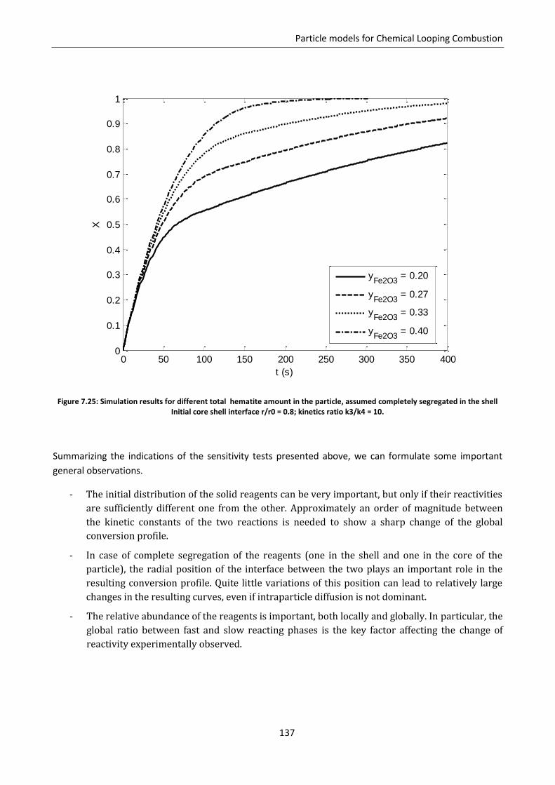
Particle models for Chemical Looping Combustion
137
Figure 7.25: Simulation results for different total hematite amount in the particle, assumed completely segregated in the shell Initial core shell interface r/r0 = 0.8; kinetics ratio k3/k4 = 10.
Summarizing the indications of the sensitivity tests presented above, we can formulate some important
general observations.
- The initial distribution of the solid reagents can be very important, but only if their reactivities
are sufficiently different one from the other. Approximately an order of magnitude between
the kinetic constants of the two reactions is needed to show a sharp change of the global
conversion profile.
- In case of complete segregation of the reagents (one in the shell and one in the core of the
particle), the radial position of the interface between the two plays an important role in the
resulting conversion profile. Quite little variations of this position can lead to relatively large
changes in the resulting curves, even if intraparticle diffusion is not dominant.
- The relative abundance of the reagents is important, both locally and globally. In particular, the
global ratio between fast and slow reacting phases is the key factor affecting the change of
reactivity experimentally observed.
0 50 100 150 200 250 300 350 4000
0.1
0.2
0.3
0.4
0.5
0.6
0.7
0.8
0.9
1
t (s)
X
yFe2O3
= 0.20
yFe2O3
= 0.27
yFe2O3
= 0.33
yFe2O3
= 0.40
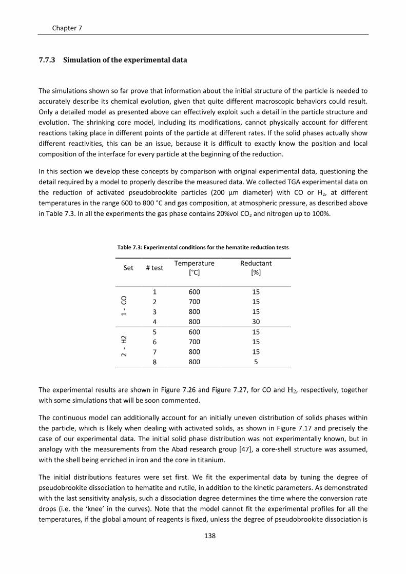
Chapter 7
138
7.7.3 Simulation of the experimental data
The simulations shown so far prove that information about the initial structure of the particle is needed to
accurately describe its chemical evolution, given that quite different macroscopic behaviors could result.
Only a detailed model as presented above can effectively exploit such a detail in the particle structure and
evolution. The shrinking core model, including its modifications, cannot physically account for different
reactions taking place in different points of the particle at different rates. If the solid phases actually show
different reactivities, this can be an issue, because it is difficult to exactly know the position and local
composition of the interface for every particle at the beginning of the reduction.
In this section we develop these concepts by comparison with original experimental data, questioning the
detail required by a model to properly describe the measured data. We collected TGA experimental data on
the reduction of activated pseudobrookite particles (200 µm diameter) with CO or H2, at different
temperatures in the range 600 to 800 °C and gas composition, at atmospheric pressure, as described above
in Table 7.3. In all the experiments the gas phase contains 20%vol CO2 and nitrogen up to 100%.
Table 7.3: Experimental conditions for the hematite reduction tests
Set # test Temperature
[°C] Reductant
[%]
1 -
CO
1 600 15
2 700 15
3 800 15
4 800 30
2 -
H2
5 600 15
6 700 15
7 800 15
8 800 5
The experimental results are shown in Figure 7.26 and Figure 7.27, for CO and H2, respectively, together
with some simulations that will be soon commented.
The continuous model can additionally account for an initially uneven distribution of solids phases within
the particle, which is likely when dealing with activated solids, as shown in Figure 7.17 and precisely the
case of our experimental data. The initial solid phase distribution was not experimentally known, but in
analogy with the measurements from the Abad research group [47], a core-shell structure was assumed,
with the shell being enriched in iron and the core in titanium.
The initial distributions features were set first. We fit the experimental data by tuning the degree of
pseudobrookite dissociation to hematite and rutile, in addition to the kinetic parameters. As demonstrated
with the last sensitivity analysis, such a dissociation degree determines the time where the conversion rate
drops (i.e. the ‘knee’ in the curves). Note that the model cannot fit the experimental profiles for all the
temperatures, if the global amount of reagents is fixed, unless the degree of pseudobrookite dissociation is
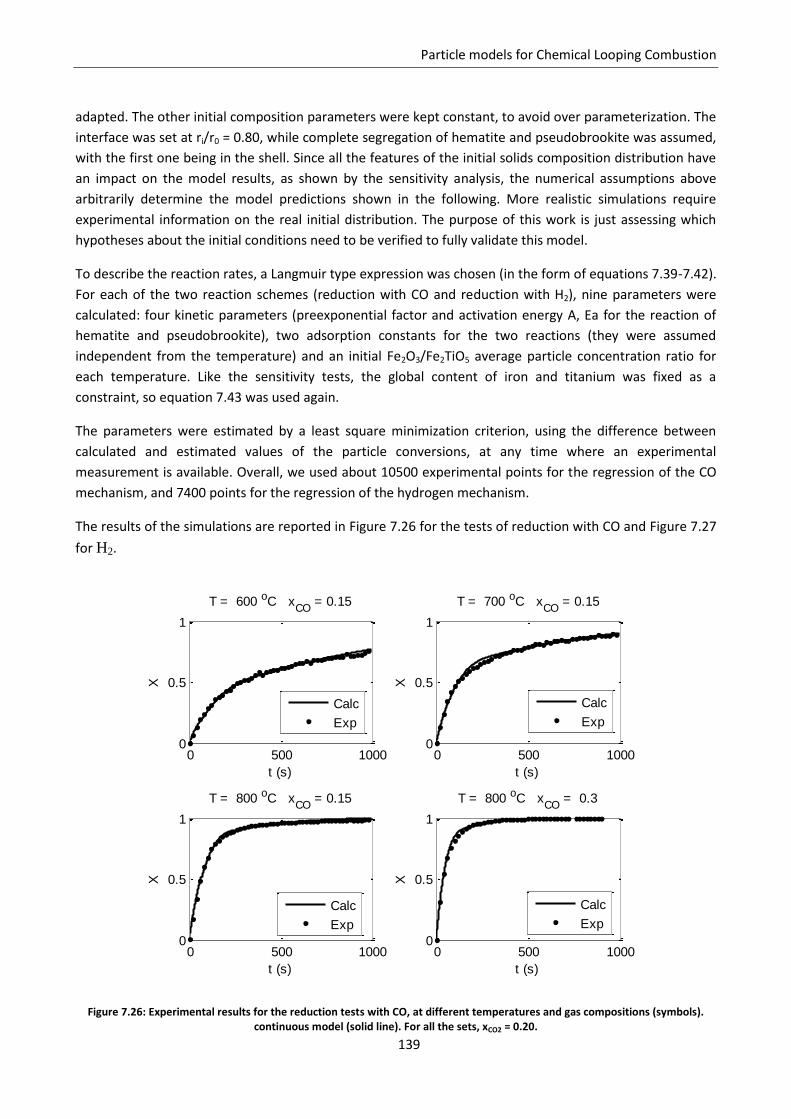
Particle models for Chemical Looping Combustion
139
adapted. The other initial composition parameters were kept constant, to avoid over parameterization. The
interface was set at ri/r0 = 0.80, while complete segregation of hematite and pseudobrookite was assumed,
with the first one being in the shell. Since all the features of the initial solids composition distribution have
an impact on the model results, as shown by the sensitivity analysis, the numerical assumptions above
arbitrarily determine the model predictions shown in the following. More realistic simulations require
experimental information on the real initial distribution. The purpose of this work is just assessing which
hypotheses about the initial conditions need to be verified to fully validate this model.
To describe the reaction rates, a Langmuir type expression was chosen (in the form of equations 7.39-7.42).
For each of the two reaction schemes (reduction with CO and reduction with H2), nine parameters were
calculated: four kinetic parameters (preexponential factor and activation energy A, Ea for the reaction of
hematite and pseudobrookite), two adsorption constants for the two reactions (they were assumed
independent from the temperature) and an initial Fe2O3/Fe2TiO5 average particle concentration ratio for
each temperature. Like the sensitivity tests, the global content of iron and titanium was fixed as a
constraint, so equation 7.43 was used again.
The parameters were estimated by a least square minimization criterion, using the difference between
calculated and estimated values of the particle conversions, at any time where an experimental
measurement is available. Overall, we used about 10500 experimental points for the regression of the CO
mechanism, and 7400 points for the regression of the hydrogen mechanism.
The results of the simulations are reported in Figure 7.26 for the tests of reduction with CO and Figure 7.27
for H2.
Figure 7.26: Experimental results for the reduction tests with CO, at different temperatures and gas compositions (symbols). continuous model (solid line). For all the sets, xCO2 = 0.20.
0 500 10000
0.5
1
t (s)
X
T = 600 oC xCO
= 0.15
Calc
Exp
0 500 10000
0.5
1
t (s)
X
T = 700 oC xCO
= 0.15
Calc
Exp
0 500 10000
0.5
1
t (s)
X
T = 800 oC xCO
= 0.15
Calc
Exp
0 500 10000
0.5
1
t (s)
X
T = 800 oC xCO
= 0.3
Calc
Exp
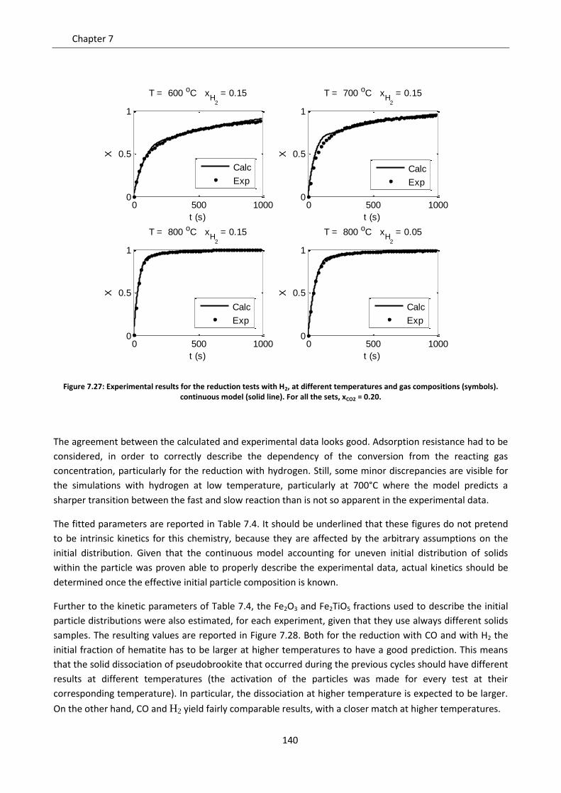
Chapter 7
140
Figure 7.27: Experimental results for the reduction tests with H2, at different temperatures and gas compositions (symbols). continuous model (solid line). For all the sets, xCO2 = 0.20.
The agreement between the calculated and experimental data looks good. Adsorption resistance had to be
considered, in order to correctly describe the dependency of the conversion from the reacting gas
concentration, particularly for the reduction with hydrogen. Still, some minor discrepancies are visible for
the simulations with hydrogen at low temperature, particularly at 700°C where the model predicts a
sharper transition between the fast and slow reaction than is not so apparent in the experimental data.
The fitted parameters are reported in Table 7.4. It should be underlined that these figures do not pretend
to be intrinsic kinetics for this chemistry, because they are affected by the arbitrary assumptions on the
initial distribution. Given that the continuous model accounting for uneven initial distribution of solids
within the particle was proven able to properly describe the experimental data, actual kinetics should be
determined once the effective initial particle composition is known.
Further to the kinetic parameters of Table 7.4, the Fe2O3 and Fe2TiO5 fractions used to describe the initial
particle distributions were also estimated, for each experiment, given that they use always different solids
samples. The resulting values are reported in Figure 7.28. Both for the reduction with CO and with H2 the
initial fraction of hematite has to be larger at higher temperatures to have a good prediction. This means
that the solid dissociation of pseudobrookite that occurred during the previous cycles should have different
results at different temperatures (the activation of the particles was made for every test at their
corresponding temperature). In particular, the dissociation at higher temperature is expected to be larger.
On the other hand, CO and H2 yield fairly comparable results, with a closer match at higher temperatures.
0 500 10000
0.5
1
t (s)
X
T = 600 oC xH
2
= 0.15
Calc
Exp
0 500 10000
0.5
1
t (s)
X
T = 700 oC xH
2
= 0.15
Calc
Exp
0 500 10000
0.5
1
t (s)
X
T = 800 oC xH
2
= 0.15
Calc
Exp
0 500 10000
0.5
1
t (s)
X
T = 800 oC xH
2
= 0.05
Calc
Exp
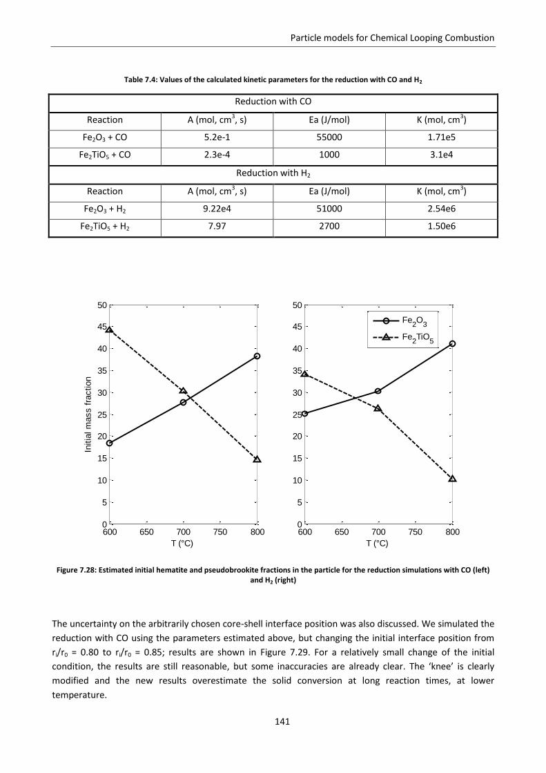
Particle models for Chemical Looping Combustion
141
Table 7.4: Values of the calculated kinetic parameters for the reduction with CO and H2
Reduction with CO
Reaction A (mol, cm3, s) Ea (J/mol) K (mol, cm3)
Fe2O3 + CO 5.2e-1 55000 1.71e5
Fe2TiO5 + CO 2.3e-4 1000 3.1e4
Reduction with H2
Reaction A (mol, cm3, s) Ea (J/mol) K (mol, cm3)
Fe2O3 + H2 9.22e4 51000 2.54e6
Fe2TiO5 + H2 7.97 2700 1.50e6
Figure 7.28: Estimated initial hematite and pseudobrookite fractions in the particle for the reduction simulations with CO (left) and H2 (right)
The uncertainty on the arbitrarily chosen core-shell interface position was also discussed. We simulated the
reduction with CO using the parameters estimated above, but changing the initial interface position from
ri/r0 = 0.80 to ri/r0 = 0.85; results are shown in Figure 7.29. For a relatively small change of the initial
condition, the results are still reasonable, but some inaccuracies are already clear. The ‘knee’ is clearly
modified and the new results overestimate the solid conversion at long reaction times, at lower
temperature.
600 650 700 750 8000
5
10
15
20
25
30
35
40
45
50
T (°C)
Initia
l m
ass f
raction
600 650 700 750 8000
5
10
15
20
25
30
35
40
45
50
T (°C)
Fe2O
3
Fe2TiO
5
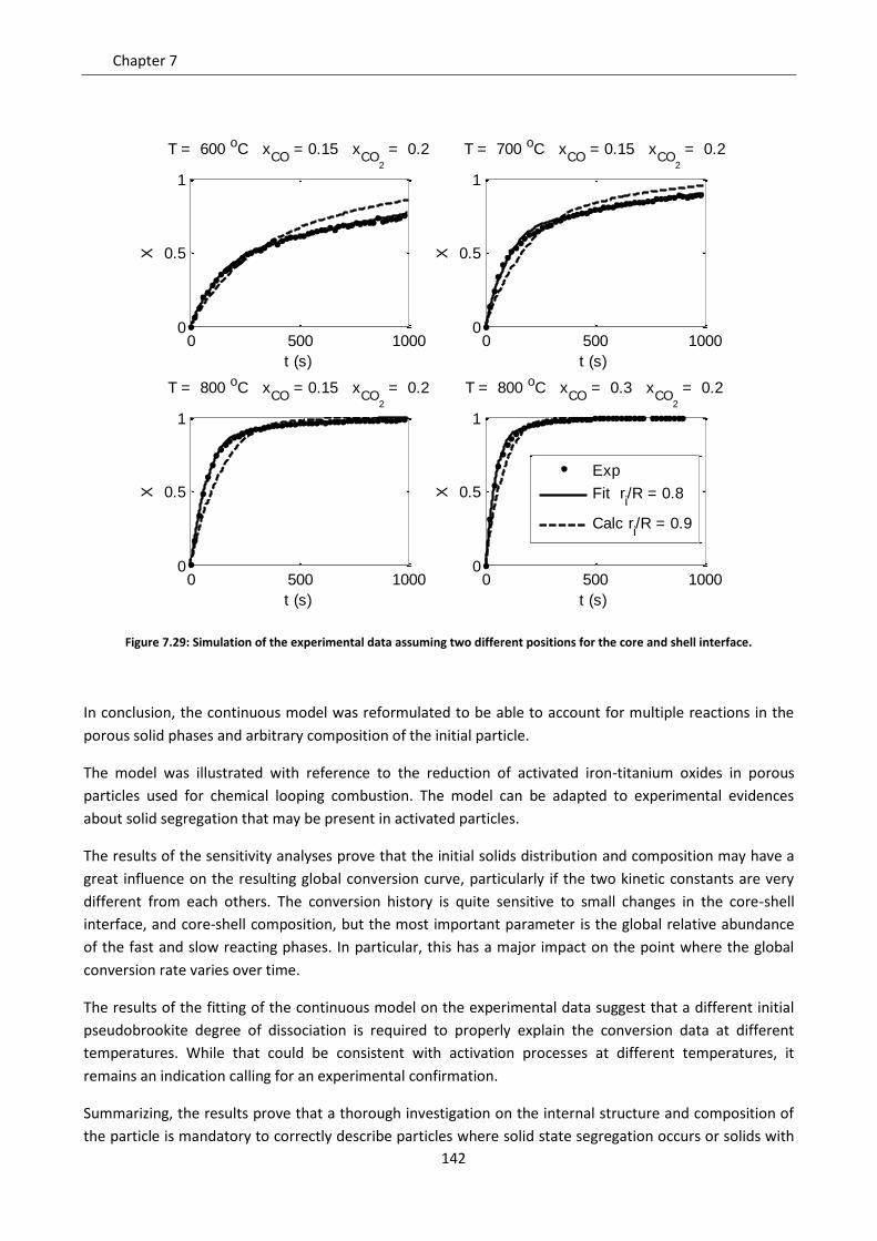
Chapter 7
142
Figure 7.29: Simulation of the experimental data assuming two different positions for the core and shell interface.
In conclusion, the continuous model was reformulated to be able to account for multiple reactions in the
porous solid phases and arbitrary composition of the initial particle.
The model was illustrated with reference to the reduction of activated iron-titanium oxides in porous
particles used for chemical looping combustion. The model can be adapted to experimental evidences
about solid segregation that may be present in activated particles.
The results of the sensitivity analyses prove that the initial solids distribution and composition may have a
great influence on the resulting global conversion curve, particularly if the two kinetic constants are very
different from each others. The conversion history is quite sensitive to small changes in the core-shell
interface, and core-shell composition, but the most important parameter is the global relative abundance
of the fast and slow reacting phases. In particular, this has a major impact on the point where the global
conversion rate varies over time.
The results of the fitting of the continuous model on the experimental data suggest that a different initial
pseudobrookite degree of dissociation is required to properly explain the conversion data at different
temperatures. While that could be consistent with activation processes at different temperatures, it
remains an indication calling for an experimental confirmation.
Summarizing, the results prove that a thorough investigation on the internal structure and composition of
the particle is mandatory to correctly describe particles where solid state segregation occurs or solids with
0 500 10000
0.5
1
t (s)
XT = 600 oC x
CO = 0.15 x
CO2
= 0.2
0 500 10000
0.5
1
t (s)
X
T = 700 oC xCO
= 0.15 xCO
2
= 0.2
0 500 10000
0.5
1
t (s)
X
T = 800 oC xCO
= 0.15 xCO
2
= 0.2
0 500 10000
0.5
1
t (s)
X
T = 800 oC xCO
= 0.3 xCO
2
= 0.2
Exp
Fit ri/R = 0.8
Calc ri/R = 0.9
Particle models for Chemical Looping Combustion
143
different reactivities are present. Data about the conversion evolution in time are extremely useful to
diagnose the global kinetics but must be supplemented by further internal characterization of the solids, to
fully characterize the intrinsic kinetics.
Notation
Pre exponential factor of Arrhenius law (mol,cm,s)
Molar concentration, of the i-th gas species, of the i-th solid species (mol/cm3)
Molar concentration of the solid i-th species in the core (mol/cm
3)
Molar concentration of the solid i-th species in the shell (mol/cm
3)
Initial molar concentration, of the i-th gas species, of the i-th solid species (mol/cm
3)
Concentration of the i-th gas species outside the particle, in bulk phase (mol/cm3)
Concentration if the i-th solid species in the j-th pore class (mol/cm
3)
Local concentration of the reacting gas species (mol/cm3)
Total concentration of gas phase, of solid phase (mol/cm3)
Heat capacity of the medium (J/cm3/K)
Heat capacity of the gas phase (J/mol/K) Size of the pores if the i-th class (cm) Effective diffusion coefficient of i used in SCM (cm
2/s)
Knudsen diffusion coefficient of the reacting gas into the pores of i-th class (cm
2/s)
Activation energy (J/mol) Fraction of solid surface occupied by the pores if i-th class Molar diffusive flux of i (mol/cm
2/s)
Superficial kinetic constant used in SCM (cm/s) Volumetric kinetic constant of the i-th reaction, used in CM (mol, cm, s) Thermal conductivity of the medium (W/cm/K) Adsorption equilibrium constant of the i-th gas species Mass of the sample in the oxidized form, in the reduced form (g) Actual mass of the sample (g) Mass of the i-th solid component into the particle (g) Molecular weight of the i-th species (g/mol) Molecular weight of the reacting gas species (g/mol) Total molar flux of the gas phase (mol/cm
2/s)
Number of discretization classes of the pore size distribution Number of gas species in the system Number of solid species in the system Radial coordinate (cm) Grain radius (cm)
Coordinate of the core-shell interface (cm) Particle radius (cm) Molar reaction rate (mol/cm
3/s)
Universal gas constant (J/mol/K)
Oxygen carrier capacity
Molar source term for the i-th gas species, for the i-th solid species (mol/cm3/s )
Molar source term for the i-th solid species in the j-th pore class (mol/cm
3/s )
Absolute temperature (K) Initial local temperature (K)
Chapter 7
144
t Time (s)
, Molar fraction of the i-th gas species, of the i-th solid species
Local conversion of the i-th solid phase Average particle conversion in the oxidation step, in the reduction step Greek letters α Sintering exponent Heat of reaction, molar based (J/mol) ԑ Porosity Thiele modulus
Stoichiometric coefficient of the i-th gas species, of the i-th solid species
Stoichiometric coefficient of the reacting gas species
Intrinsic density of the i-th solid species (g/cm3)
145
Chapter 8. Comparison between the Shrinking Core Model and the
Continuous Model
In the previous sections, different approaches to the description of non catalytic gas-solid reactions were
considered, also in comparison with real processes and experimental data. All of the presented results
proved that the quantitative treatment of reactive solids must be related to a correct description of the
actual physics, that can often be extremely complicated by:
1) The heterogeneous nature of the reaction, causing interference of chemical processes (reactions) and
transport phenomena (internal diffusion)
2) The modification of the solids structure as a consequence of its reaction.
The most rigorous approach requires solving the microscopic conservation equations for the gas and the
solid species within the single particle, with its actual texture. In practice, the porous phase is treated as
pseudo-homogeneous continuous phase, with a given porosity (constant or locally variable), and a local
concentration of accessible surface per unit volume.
Simplified approaches assume non-porous particles, or non-porous shrinking core model (SCM). The latter
is extremely popular, notwithstanding its limitations. It assumes that the reaction takes place only on a
surface, dividing the unreacted core by the product layer in the particle, and moving to the center as the
reaction goes on. This situation is realistic if the core is not porous. If the particle is completely porous, SCM
is still applicable if the reaction is fast compared to the inward diffusion of the gaseous reagent.
In the recent literature, many Authors claim the necessity to use the detailed approach [58-60], but several
still choose the shrinking core model because of its simplicity [13, 15, 16, 18]. As already mentioned in
section §2, it should be noticed that the physical description of the SCM only holds when the reaction is
very fast compared to the diffusion of the gas. On the contrary, when diffusion is fast the gas tends to be
uniformly distributed inside the particle (if the particle is initially porous), so the core-shell structure cannot
be formed. Beside this, other inconsistencies can originate from the presence of equilibrium reactions, and
multiple reaction steps.
In spite of this, the SCM can still be used, especially when an apparent value of the superficial kinetic
constant can decently fit the available experimental data. It is possible that the SCM can reasonably
approximate the same results as the continuous models, as discussed in this work and frequently stated in
the literature [61]. A comparison was made by Ishida and Wen [62], who concluded that in most cases this
approximation is good enough. In diffusive regime, Duong demonstrated [63] that the SCM and continuous
models can become mathematically identical, no matter which is the chosen expression for the reaction
rate.
Nevertheless, the limiting hypotheses implied by the shrinking core model should be a good reason not to
use it for most applications (at least when the particle is fully porous, or diffusion is not dominant). Even if
SCM can fit the experimental data, this doesn’t mean that errors cannot arise when the fitted parameters
are used to simulate conditions that are typically different from the available experimental data, if in reality
Chapter 8
146
the particle reaction doesn’t produce a core-shell structure. However, this warning is often neglected. In
this section, we investigated more deeply into the different behavior of SCM and CM at different
conditions, in order to gain more information about the safe applicability of SCM for applications involving
porous particles.
Improvements in the quantitative description of reacting porous solids require developing sub-models
accounting for the local porosity variations. Restructuring of the solids along the reaction course can affect
both the rate of internal diffusion and the surface reaction rate. Sub-models of particle sintering and
restructuring can be effectively exploited by particle models that properly describe both surface reactions
and internal diffusion, improving on simpler particle models that occasionally and partially mimic the
observed conversion evolution. In this section we started a systematic comparison of the models [64]. Here
we consider the grain and the traditional models presented in section §4 as reference cases. The study was
focused on their different behavior at different controlling regimes. The final aim was also assessing the
reliability of the SCM in simulations far away from the experimental data used to establish the apparent
kinetic constant, and the possible divergence of the SCM from the continuous model when used in non-
diffusion controlled conditions.
8.1 Description of the compared models
8.1.1 Continuous model
For the present analysis, a generic reaction is considered, in which the solid species A and the gas species B
yields a solid and a gas species through the irreversible reaction:
a A(s) + b B(g) c C(s) + d D(g) 8.1
Examples of this model chemistry are the direct reduction of iron oxides by H2 or CO, calcinations of ZnS
and FeS with O2 to give metal oxides (ZnO, Fe2O3), combustion of coal to give CO2 and ashes.
The conservation equations for the gas and solid species within a porous solid spherical particle, described
as a pseudo homogeneous phase were reported in section §4 (equations 4.37-4.41).
In most applications, the gaseous reactants are highly concentrated in the gas phase, often the unique
species (no diluents). Accordingly, the diffusive flux requires the generalized Fick law, presented in
equations 5.42-5.47, possibly including Knudsen diffusion (equation 5.93) with the effective binary diffusion
coefficients depending on the local porosity and tortuosity of the solid (equation 5.109).
Commonly, the tortuosity is considered as a parameter, whereas the porosity depends on the degree of
conversion of the solid, due to the fact that the species A and C may have different densities, in general. If
no variation of volume of the particle during the reaction is assumed, the porosity variations can be easily
calculated, thanks to equations 4.10 and 4.45.
Comparison between the Shrinking Core Model and the Continuous Model
147
A common choice of the form of the reaction rate R is described assuming irreversibility and first order in
the concentration of the gas reactant, but including a non linear function of the solid conversion X, as
follows:
8.2
8.3
Where k is the kinetic constant. As already discussed in chapter 4, f(X) describes the local abundance of
solid A per unit volume of porous solids. Being the reaction heterogeneous in nature, the relevant measure
of abundance is the amount of superficial A per unit volume, which strongly depends on the local structure
of the porous solids.
In the present work the traditional model in the form of equation 4.72 was considered. One advantage of
using it is that it can be easily extended to non spherical grain geometries, with the parameter α that can
take into account different shapes of the micrograins, and can also account for the reshaping phenomena
occurring during the reaction, namely sintering of the solid due to high temperatures. If sintering occurs, α
will become larger, because there will be a faster decrease of the superficial area at the beginning of the
reaction.
The particle model can be solved with the initial and boundary conditions of equations 4.47-4.50.
The solutions of the model are the time and space dependent concentration profiles ci(r,t) of any species.
From ci(r,t), the function X(t) can be calculated by integration. Initial radial profiles must be provided to the
model both for the gas and the solid species. These profiles can also be non uniform in r, for instance if the
particle composition is not homogeneous before starting the reaction, as it was evidenced in section §7.
8.1.1.1 Possible simplifications to the continuous model
The model presented above can rigorously simulate the evolution of the conversion of the solid particle in
isothermal conditions, provided the correct values for the parameters and the boundary and initial
conditions. The model equations can also be somehow simplified, by considering the following
assumptions:
a) The gas mixture is composed of only 2 components, B and D.
b) The molecular weights of solid species A and C are almost the same, as well as their intrinsic
densities. This allows considering the porosity as a constant.
c) The reaction is equimolar with respect to the gas phase, which means that b = d.
d) The system is isothermal and isobaric.
e) The external mass transfer is very fast, so that the concentration at the particle surface is the same
as the bulk of the gas.
f) No change of particle size occurs.
Chapter 8
148
Hypothesis a), b) and d) have an effect on the diffusive flux. If only two components are present, a binary
Fick law can be used, with a single diffusion coefficient DBD. If pressure, temperature and porosity are
constant, such a coefficient will be constant, and can be carried out of the derivative.
Hypothesis b), c) allow to neglect the convection term in the gas species conservation equations, so that
the total concentration balance 4.38 doesn’t need to be solved. In fact, the sum of the molar production
rates of the gas is zero if the reaction is equimolar. Besides, there is no convection induced by a change in
the porosity, which can change the volume occupied by the gas. Actually, the porosity time derivative in
4.37 is usually not important even if hypothesis b) is not verified.
In these conditions, we can write the equations for gas reagent B as:
8.4
And for the solid reactant A:
8.5
Also the boundary conditions can be simplified, by using condition e).
8.6
8.7
8.8
Equations 8.4-8.5 can also be reformulated in non-dimensional form, as follows:
8.9
8.10
Where the non-dimensional variables are defined as:
8.11
And the following non-dimensional numbers are introduced:
8.12
Comparison between the Shrinking Core Model and the Continuous Model
149
Where t* is the time for having full conversion of the particle. is the Thiele modulus, so its value
quantifies the ratio between the kinetic and diffusive resistance. The boundary conditions in non
dimensional form are:
8.13
8.14
8.15
This version of the continuous model was chosen to carry out a comparison with SCM. Although the
simplifications introduced to derive such a simplified CM are quite relevant, our aim is comparing SCM and
CM in the conditions where the two models are closer (same diffusion model, same transport phenomena,
same effective diffusivities, same kinetic scheme). As shown below, differences in the numerical results can
be dramatic.
8.1.2 Shrinking core model
The same gas solid reaction can be described with a shrinking core model. It assumes that the reaction is
localized at an interface r*, moving from the external surface of the particle to its center as long as the
reaction goes on. It is deduced by solving the equations for the gas reactant, where the reaction is a
boundary condition at the core-shell interface, and only diffusion occurs in the layer between the reaction
interface and the external particle surface. The model details are described in section §2.
For the considered stoichiometry (equation 8.1), the balance describing the evolution of the reagent solid A
becomes as follows:
8.16
Or, in terms of conversion X:
8.17
Note that equation 8.17 is very similar to the equation of the complete grain model (equation 4.70). The
grain model is in fact an application of the shrinking core model to the grain scale, and the two models
become eventually equivalent if a0 = 3/r0 (the initial surface-volume ratio of the solid in equal to the surface
area of the particle), and k = a0k’. If the concentration of B at the pellet surface is constant in time, as well
as the system temperature, the equation has an analytical solution, quite simple as t(X):
Chapter 8
150
8.18
8.19
8.20
In this formulation, τK and τD quantify the importance of the kinetic and internal diffusion resistances
respectively.
In non-dimensional form:
8.21
A Thiele modulus can also be defined for the SCM, which is directly related to the ratio between the two
characteristic times τK and τD:
8.22
Equation 8.21 for the two regimes becomes:
8.23
8.24
These expressions are independent from the values of the parameters (τK and τD will have an effect on the
actual non normalized time scale). They are also the two asymptotic profiles, in the sense that any other
curve in the intermediate regime will lay in between the two.
In order to quantify how well a shrinking core model can numerically approximate a continuous model, the
comparison with a simplified generalized grain model will be considered. It is true that some of the degree
of detail that a fully rigorous continuous model can offer is lost in the simplified version (equations 8.9-
8.10), and sometimes some of the hypothesis mentioned are not verified. Yet, this comparison is quite
useful because it concerns the non analytical model closest to the shrinking core, and so it can be a good
indication whether it is necessary or not to use a continuous model, instead of a shrinking core that could
approximate its same solution. The effect of natural convection, change of porosity, temperature and
external mass transfer can add further differences between the two approaches, and each of these should
be analyzed individually, as it was proved in section §6.
Even more complications can originate when considering multiple reactions, possibly reversible. The
present comparison is focused on the effect of sintering, expressed by the parameter α, and the effect of
the controlling regime. Further, we aim at spotting those circumstances in which the two models may give
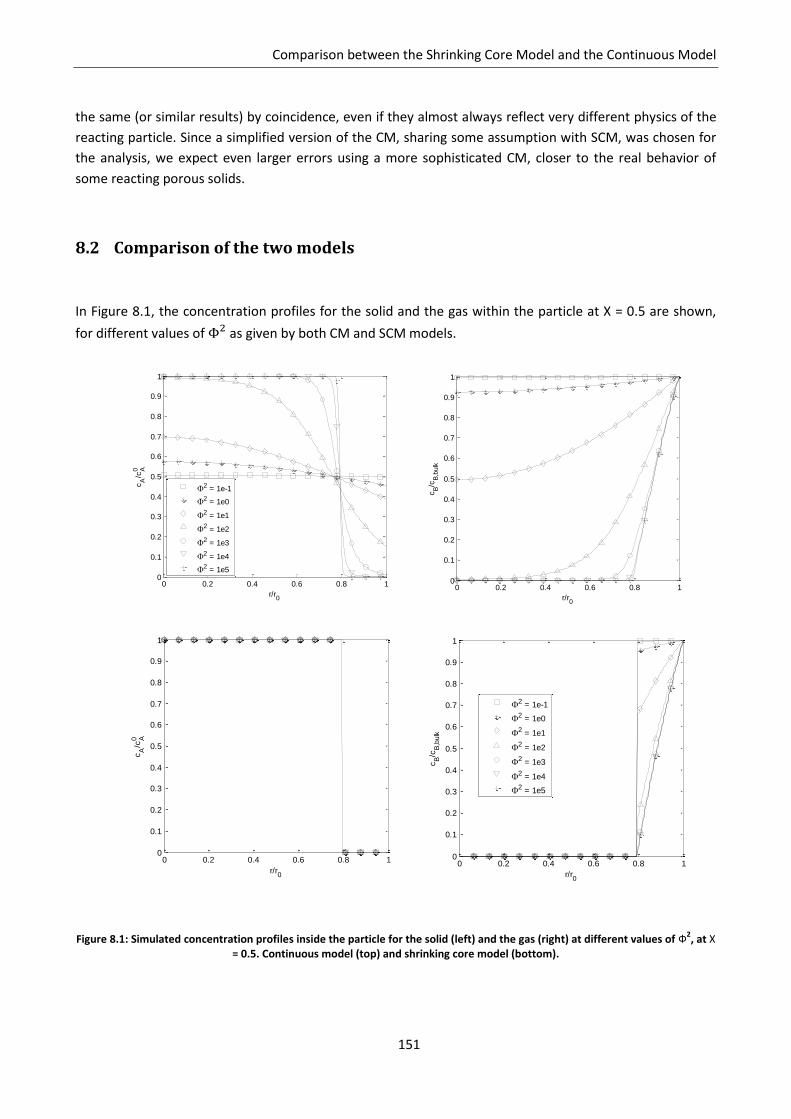
Comparison between the Shrinking Core Model and the Continuous Model
151
the same (or similar results) by coincidence, even if they almost always reflect very different physics of the
reacting particle. Since a simplified version of the CM, sharing some assumption with SCM, was chosen for
the analysis, we expect even larger errors using a more sophisticated CM, closer to the real behavior of
some reacting porous solids.
8.2 Comparison of the two models
In Figure 8.1, the concentration profiles for the solid and the gas within the particle at X = 0.5 are shown,
for different values of as given by both CM and SCM models.
Figure 8.1: Simulated concentration profiles inside the particle for the solid (left) and the gas (right) at different values of Ф2, at X
= 0.5. Continuous model (top) and shrinking core model (bottom).
0 0.2 0.4 0.6 0.8 10
0.1
0.2
0.3
0.4
0.5
0.6
0.7
0.8
0.9
1
r/r0
cA
/cA0
0 0.2 0.4 0.6 0.8 10
0.1
0.2
0.3
0.4
0.5
0.6
0.7
0.8
0.9
1
r/r0
cB/c
B,b
ulk
2 = 1e-1
2 = 1e0
2 = 1e1
2 = 1e2
2 = 1e3
2 = 1e4
2 = 1e5
0 0.2 0.4 0.6 0.8 10
0.1
0.2
0.3
0.4
0.5
0.6
0.7
0.8
0.9
1
r/r0
cA
/cA0
0 0.2 0.4 0.6 0.8 10
0.1
0.2
0.3
0.4
0.5
0.6
0.7
0.8
0.9
1
r/r0
cB/c
B,b
ulk
2 = 1e-1
2 = 1e0
2 = 1e1
2 = 1e2
2 = 1e3
2 = 1e4
2 = 1e5
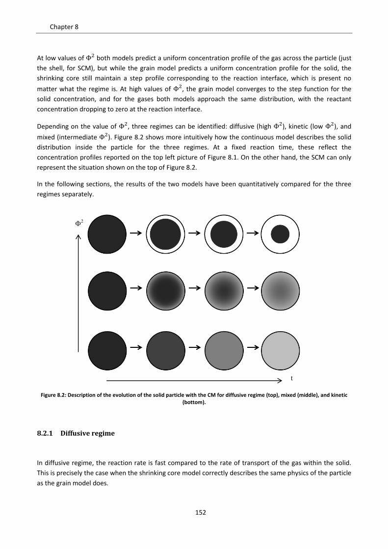
Chapter 8
152
At low values of both models predict a uniform concentration profile of the gas across the particle (just
the shell, for SCM), but while the grain model predicts a uniform concentration profile for the solid, the
shrinking core still maintain a step profile corresponding to the reaction interface, which is present no
matter what the regime is. At high values of , the grain model converges to the step function for the
solid concentration, and for the gases both models approach the same distribution, with the reactant
concentration dropping to zero at the reaction interface.
Depending on the value of , three regimes can be identified: diffusive (high ), kinetic (low ), and
mixed (intermediate ). Figure 8.2 shows more intuitively how the continuous model describes the solid
distribution inside the particle for the three regimes. At a fixed reaction time, these reflect the
concentration profiles reported on the top left picture of Figure 8.1. On the other hand, the SCM can only
represent the situation shown on the top of Figure 8.2.
In the following sections, the results of the two models have been quantitatively compared for the three
regimes separately.
Figure 8.2: Description of the evolution of the solid particle with the CM for diffusive regime (top), mixed (middle), and kinetic (bottom).
8.2.1 Diffusive regime
In diffusive regime, the reaction rate is fast compared to the rate of transport of the gas within the solid.
This is precisely the case when the shrinking core model correctly describes the same physics of the particle
as the grain model does.
t
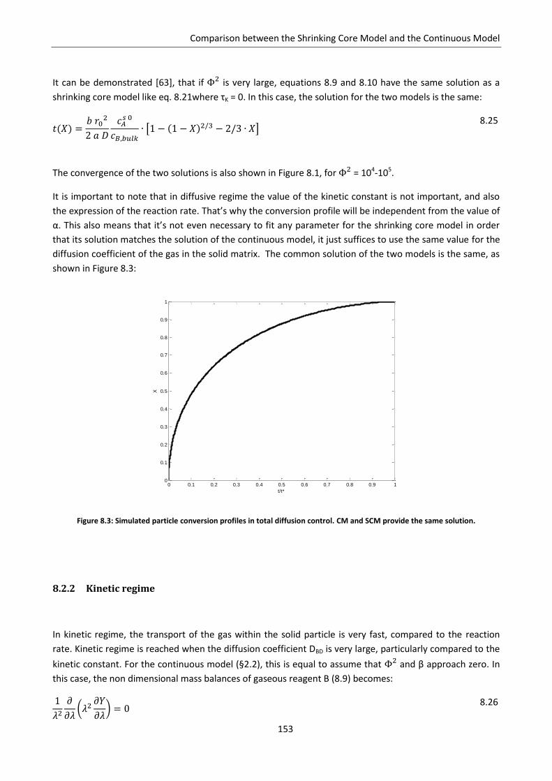
Comparison between the Shrinking Core Model and the Continuous Model
153
It can be demonstrated [63], that if is very large, equations 8.9 and 8.10 have the same solution as a
shrinking core model like eq. 8.21where τK = 0. In this case, the solution for the two models is the same:
8.25
The convergence of the two solutions is also shown in Figure 8.1, for = 104-105.
It is important to note that in diffusive regime the value of the kinetic constant is not important, and also
the expression of the reaction rate. That’s why the conversion profile will be independent from the value of
α. This also means that it’s not even necessary to fit any parameter for the shrinking core model in order
that its solution matches the solution of the continuous model, it just suffices to use the same value for the
diffusion coefficient of the gas in the solid matrix. The common solution of the two models is the same, as
shown in Figure 8.3:
Figure 8.3: Simulated particle conversion profiles in total diffusion control. CM and SCM provide the same solution.
8.2.2 Kinetic regime
In kinetic regime, the transport of the gas within the solid particle is very fast, compared to the reaction
rate. Kinetic regime is reached when the diffusion coefficient DBD is very large, particularly compared to the
kinetic constant. For the continuous model (§2.2), this is equal to assume that and β approach zero. In
this case, the non dimensional mass balances of gaseous reagent B (8.9) becomes:
8.26
0 0.1 0.2 0.3 0.4 0.5 0.6 0.7 0.8 0.9 10
0.1
0.2
0.3
0.4
0.5
0.6
0.7
0.8
0.9
1
t/t*
X
Chapter 8
154
With the boundary conditions:
8.27
8.28
The solution is Y = 1 for any normalized radius, λ. This means that the concentration of B is equal to the
bulk concentration in any point of the pellet. In the case of a classical grain model (α = 2/3), the
concentration balance for the solid reactant A becomes:
8.29
In terms of conversion:
8.30
So that the continuous model has analytical solution as well, if cB,bulk is constant in time:
8.31
In kinetic regime, the SCM solution can be obtained by considering τD = 0 in equation 8.21:
8.32
Comparing the results of equation 8.31 and 8.32, we see that they are identical when we set:
8.33
So the superficial kinetic constant for the shrinking core model is equal to the volumetric kinetic constant of
the continuous model, divided by the surface-to-volume ratio of the whole particle. In other words, the
product between the superficial constants of the two models and their respective initial superficial areas of
the solid reacting phase is the same. Note that this is true only because the grain model is applied.
It is interesting to point out that the analogy of solutions is a coincidence. In fact the two models are
physically describing two completely different situations: on the one hand, the shrinking core simulates a
single macro particle, with the solid A converting from the external surface to the core. On the other one,
the continuous model describes a particle reacting homogeneously along the radial coordinate. The
numerical results of the two are, however, precisely the same. This is because the grain model is actually
representing a number of micrograins, with all the same size and all reacting like shrinking cores with the
same rate, because the concentration of the gas is the same in any point of the macro pellet.
Comparison between the Shrinking Core Model and the Continuous Model
155
8.2.2.1 Study for a generic value of α
We now investigate the extent of adaptation of SCM to the classical grain model (α = 2/3). If we consider a
general expression of the superficial area of the reacting species as a function of the conversion within the
continuous model:
8.34
We obtain the generalized grain model. In kinetic regime that leads to:
8.35
Which can be analytically integrated as well, giving:
8.36
We can evaluate how close the shrinking core model can approach the continuous model in a kinetic
regime, depending on α, by considering the difference of the two t(X) analytical solutions, 8.32 and 8.36:
8.37
The kinetic constant k’ by which the SCM best approximates the continuous model can be estimated by
least squares criteria, requesting the best match between tCM and tSCM over the whole range of conversion:
8.38
Substituting equation 8.37 into 8.38, calculating the derivative and solving the equation in k’ we obtain:
8.39
It is trivial to see that, if α = 2/3, equation 8.39 reduces to equation 8.33. Note that k’opt in the least squares
sense does not imply a coincidence of t(X) for both models at any X value.
Note that, for α > 1, the function described by equation 8.36 diverges for X-->1, suggesting that the integral
of equation 8.38 might not converge. However, carrying out the algebra we find that the error function
given by the integral is finite, except for α=3/2, 2, 7/3:
8.40
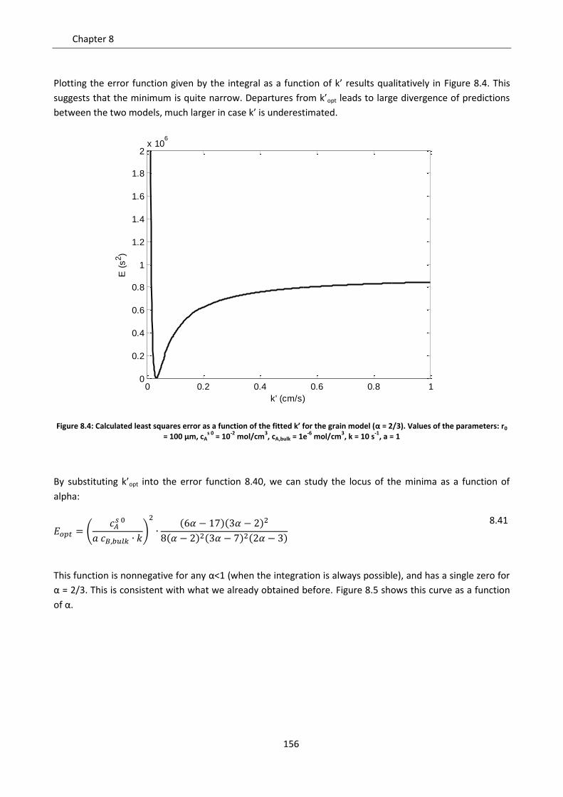
Chapter 8
156
Plotting the error function given by the integral as a function of k’ results qualitatively in Figure 8.4. This
suggests that the minimum is quite narrow. Departures from k’opt leads to large divergence of predictions
between the two models, much larger in case k’ is underestimated.
Figure 8.4: Calculated least squares error as a function of the fitted k’ for the grain model (α = 2/3). Values of the parameters: r0 = 100 μm, cA
s 0 = 10
-2 mol/cm
3, cA,bulk = 1e
-6 mol/cm
3, k = 10 s
-1, a = 1
By substituting k’opt into the error function 8.40, we can study the locus of the minima as a function of
alpha:
8.41
This function is nonnegative for any α<1 (when the integration is always possible), and has a single zero for
α = 2/3. This is consistent with what we already obtained before. Figure 8.5 shows this curve as a function
of α.
0 0.2 0.4 0.6 0.8 10
0.2
0.4
0.6
0.8
1
1.2
1.4
1.6
1.8
2x 10
6
k' (cm/s)
E (
s2)
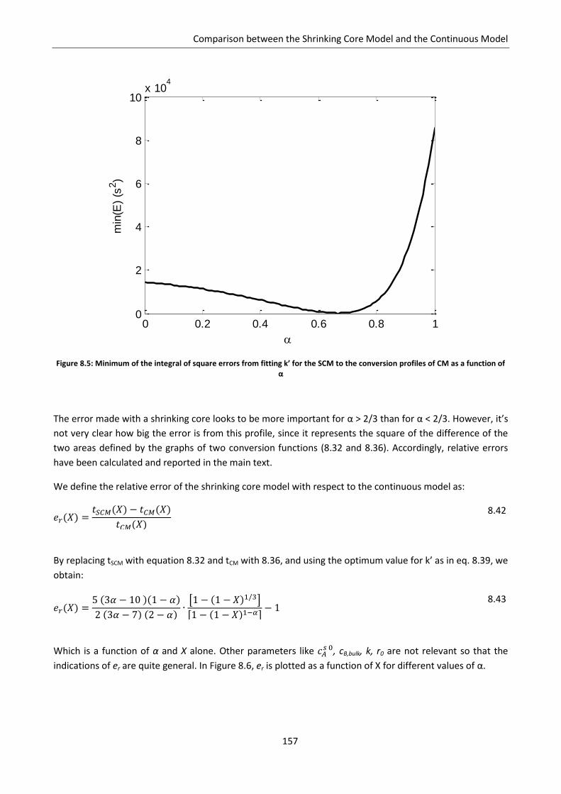
Comparison between the Shrinking Core Model and the Continuous Model
157
Figure 8.5: Minimum of the integral of square errors from fitting k’ for the SCM to the conversion profiles of CM as a function of α
The error made with a shrinking core looks to be more important for α > 2/3 than for α < 2/3. However, it’s
not very clear how big the error is from this profile, since it represents the square of the difference of the
two areas defined by the graphs of two conversion functions (8.32 and 8.36). Accordingly, relative errors
have been calculated and reported in the main text.
We define the relative error of the shrinking core model with respect to the continuous model as:
8.42
By replacing tSCM with equation 8.32 and tCM with 8.36, and using the optimum value for k’ as in eq. 8.39, we
obtain:
8.43
Which is a function of α and X alone. Other parameters like , cB,bulk, k, r0 are not relevant so that the
indications of er are quite general. In Figure 8.6, er is plotted as a function of X for different values of α.
0 0.2 0.4 0.6 0.8 10
2
4
6
8
10x 10
4
min
(E)
(s2)
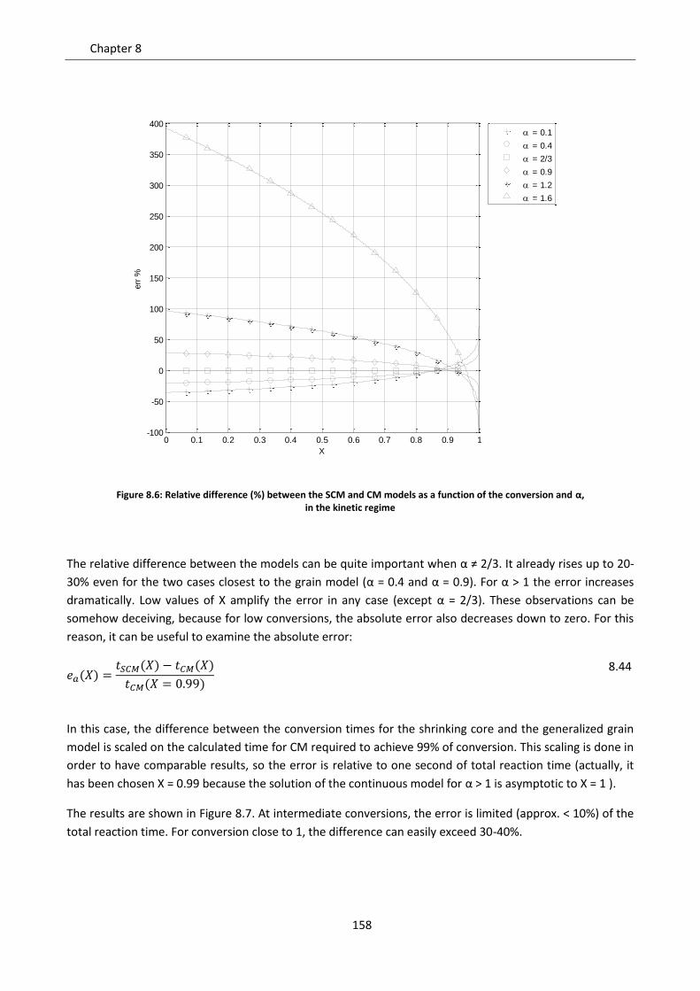
Chapter 8
158
Figure 8.6: Relative difference (%) between the SCM and CM models as a function of the conversion and α, in the kinetic regime
The relative difference between the models can be quite important when α ≠ 2/3. It already rises up to 20-
30% even for the two cases closest to the grain model (α = 0.4 and α = 0.9). For α > 1 the error increases
dramatically. Low values of X amplify the error in any case (except α = 2/3). These observations can be
somehow deceiving, because for low conversions, the absolute error also decreases down to zero. For this
reason, it can be useful to examine the absolute error:
8.44
In this case, the difference between the conversion times for the shrinking core and the generalized grain
model is scaled on the calculated time for CM required to achieve 99% of conversion. This scaling is done in
order to have comparable results, so the error is relative to one second of total reaction time (actually, it
has been chosen X = 0.99 because the solution of the continuous model for α > 1 is asymptotic to X = 1 ).
The results are shown in Figure 8.7. At intermediate conversions, the error is limited (approx. < 10%) of the
total reaction time. For conversion close to 1, the difference can easily exceed 30-40%.
0 0.1 0.2 0.3 0.4 0.5 0.6 0.7 0.8 0.9 1-100
-50
0
50
100
150
200
250
300
350
400
X
err
%
= 0.1
= 0.4
= 2/3
= 0.9
= 1.2
= 1.6
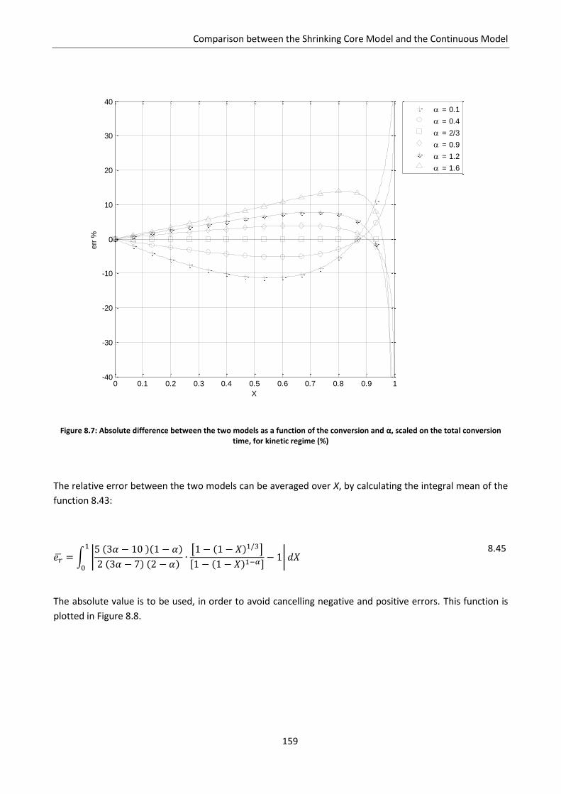
Comparison between the Shrinking Core Model and the Continuous Model
159
Figure 8.7: Absolute difference between the two models as a function of the conversion and α, scaled on the total conversion time, for kinetic regime (%)
The relative error between the two models can be averaged over X, by calculating the integral mean of the
function 8.43:
8.45
The absolute value is to be used, in order to avoid cancelling negative and positive errors. This function is
plotted in Figure 8.8.
0 0.1 0.2 0.3 0.4 0.5 0.6 0.7 0.8 0.9 1-40
-30
-20
-10
0
10
20
30
40
X
err
%
= 0.1
= 0.4
= 2/3
= 0.9
= 1.2
= 1.6
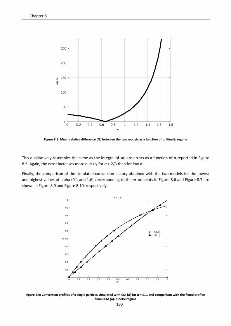
Chapter 8
160
Figure 8.8: Mean relative difference (%) between the two models as a function of α. Kinetic regime
This qualitatively resembles the same as the integral of square errors as a function of α reported in Figure
8.5. Again, the error increases more quickly for α > 2/3 than for low α.
Finally, the comparison of the simulated conversion history obtained with the two models for the lowest
and highest values of alpha (0.1 and 1.6) corresponding to the errors plots in Figure 8.6 and Figure 8.7 are
shown in Figure 8.9 and Figure 8.10, respectively.
Figure 8.9: Conversion profiles of a single particle, simulated with CM (Δ) for α = 0.1, and comparison with the fitted profiles from SCM (o). Kinetic regime
0 0.2 0.4 0.6 0.8 1 1.2 1.4 1.6 1.80
50
100
150
200
250
err
%
0 0.1 0.2 0.3 0.4 0.5 0.6 0.7 0.8 0.9 10
0.1
0.2
0.3
0.4
0.5
0.6
0.7
0.8
0.9
1
t/t*
X
= 0.10
SCM
CM
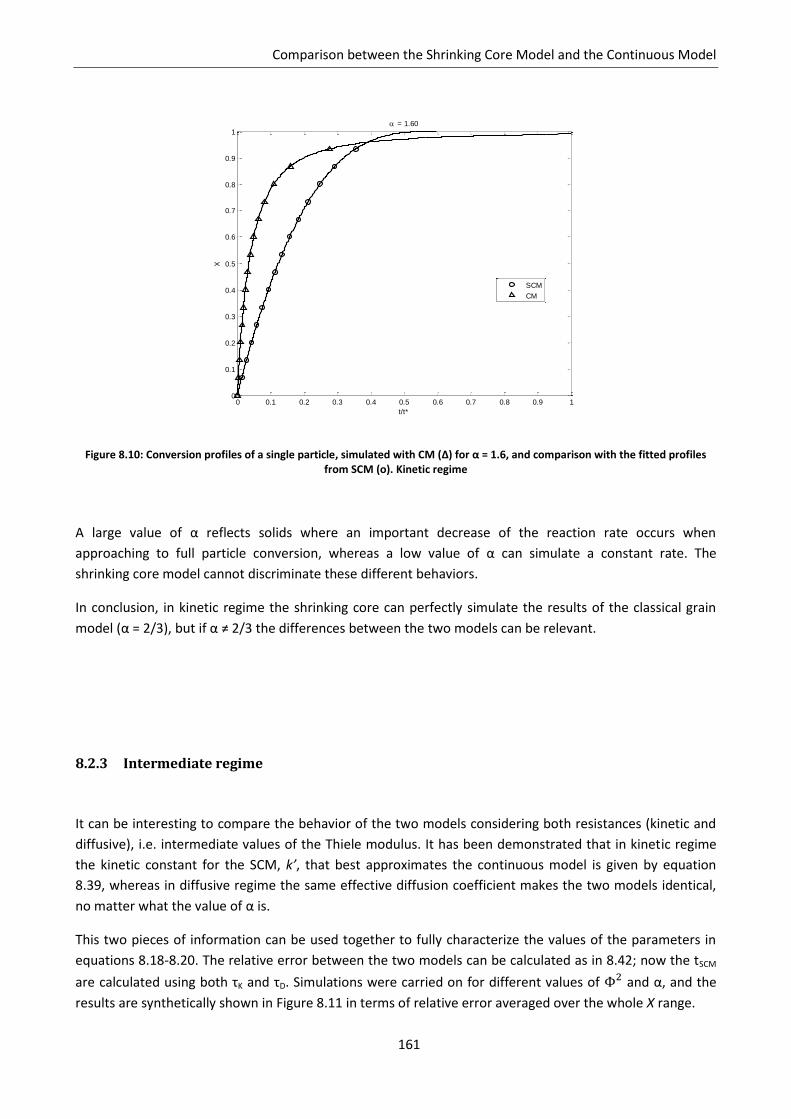
Comparison between the Shrinking Core Model and the Continuous Model
161
Figure 8.10: Conversion profiles of a single particle, simulated with CM (Δ) for α = 1.6, and comparison with the fitted profiles from SCM (o). Kinetic regime
A large value of α reflects solids where an important decrease of the reaction rate occurs when
approaching to full particle conversion, whereas a low value of α can simulate a constant rate. The
shrinking core model cannot discriminate these different behaviors.
In conclusion, in kinetic regime the shrinking core can perfectly simulate the results of the classical grain
model (α = 2/3), but if α ≠ 2/3 the differences between the two models can be relevant.
8.2.3 Intermediate regime
It can be interesting to compare the behavior of the two models considering both resistances (kinetic and
diffusive), i.e. intermediate values of the Thiele modulus. It has been demonstrated that in kinetic regime
the kinetic constant for the SCM, k’, that best approximates the continuous model is given by equation
8.39, whereas in diffusive regime the same effective diffusion coefficient makes the two models identical,
no matter what the value of α is.
This two pieces of information can be used together to fully characterize the values of the parameters in
equations 8.18-8.20. The relative error between the two models can be calculated as in 8.42; now the tSCM
are calculated using both τK and τD. Simulations were carried on for different values of and α, and the
results are synthetically shown in Figure 8.11 in terms of relative error averaged over the whole X range.
0 0.1 0.2 0.3 0.4 0.5 0.6 0.7 0.8 0.9 10
0.1
0.2
0.3
0.4
0.5
0.6
0.7
0.8
0.9
1
t/t*
X
= 1.60
SCM
CM
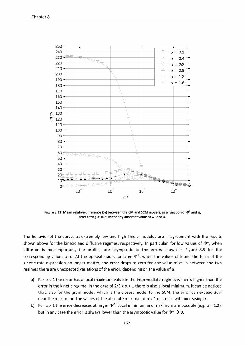
Chapter 8
162
Figure 8.11: Mean relative difference (%) between the CM and SCM models, as a function of Ф2 and α,
after fitting k’ in SCM for any different value of Ф2 and α.
The behavior of the curves at extremely low and high Thiele modulus are in agreement with the results
shown above for the kinetic and diffusive regimes, respectively. In particular, for low values of , when
diffusion is not important, the profiles are asymptotic to the errors shown in Figure 8.5 for the
corresponding values of α. At the opposite side, for large , when the values of k and the form of the
kinetic rate expression no longer matter, the error drops to zero for any value of α. In between the two
regimes there are unexpected variations of the error, depending on the value of α.
a) For α < 1 the error has a local maximum value in the intermediate regime, which is higher than the
error in the kinetic regime. In the case of 2/3 < α < 1 there is also a local minimum. It can be noticed
that, also for the grain model, which is the closest model to the SCM, the error can exceed 20%
near the maximum. The values of the absolute maxima for α < 1 decrease with increasing α.
b) For α > 1 the error decreases at larger . Local minimum and maximum are possible (e.g. α = 1.2),
but in any case the error is always lower than the asymptotic value for 0.
10-2
100
102
104
0
10
20
30
40
50
60
70
80
90
100
110
120
130
140
150
160
170
180
190
200
210
220
230
240
250
2
err
%
= 0.1
= 0.4
= 2/3
= 0.9
= 1.2
= 1.6
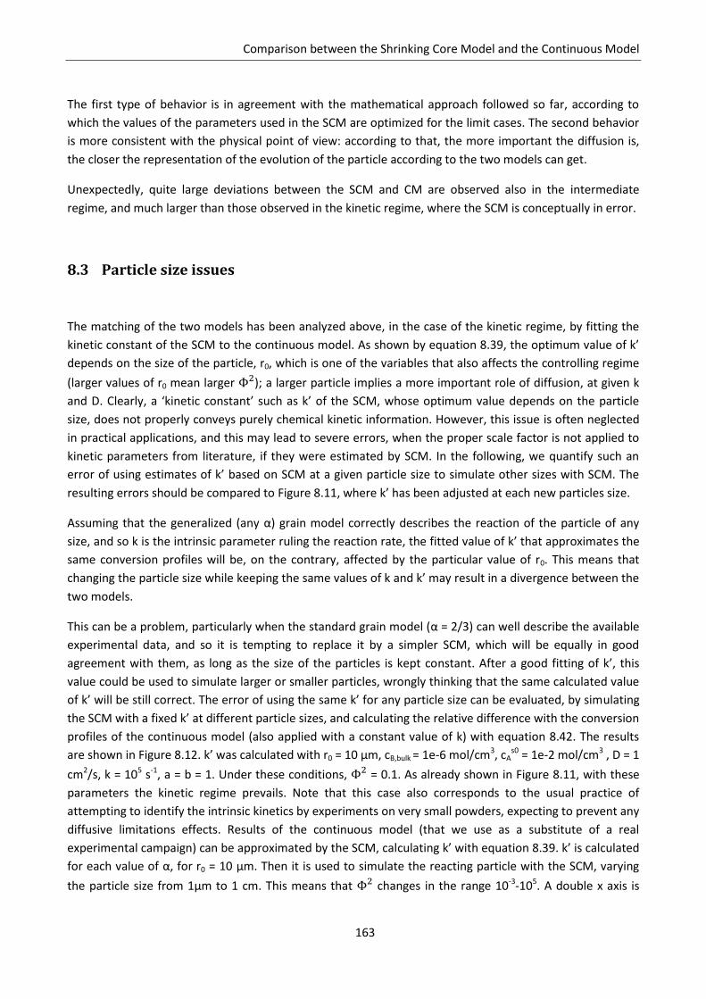
Comparison between the Shrinking Core Model and the Continuous Model
163
The first type of behavior is in agreement with the mathematical approach followed so far, according to
which the values of the parameters used in the SCM are optimized for the limit cases. The second behavior
is more consistent with the physical point of view: according to that, the more important the diffusion is,
the closer the representation of the evolution of the particle according to the two models can get.
Unexpectedly, quite large deviations between the SCM and CM are observed also in the intermediate
regime, and much larger than those observed in the kinetic regime, where the SCM is conceptually in error.
8.3 Particle size issues
The matching of the two models has been analyzed above, in the case of the kinetic regime, by fitting the
kinetic constant of the SCM to the continuous model. As shown by equation 8.39, the optimum value of k’
depends on the size of the particle, r0, which is one of the variables that also affects the controlling regime
(larger values of r0 mean larger ); a larger particle implies a more important role of diffusion, at given k
and D. Clearly, a ‘kinetic constant’ such as k’ of the SCM, whose optimum value depends on the particle
size, does not properly conveys purely chemical kinetic information. However, this issue is often neglected
in practical applications, and this may lead to severe errors, when the proper scale factor is not applied to
kinetic parameters from literature, if they were estimated by SCM. In the following, we quantify such an
error of using estimates of k’ based on SCM at a given particle size to simulate other sizes with SCM. The
resulting errors should be compared to Figure 8.11, where k’ has been adjusted at each new particles size.
Assuming that the generalized (any α) grain model correctly describes the reaction of the particle of any
size, and so k is the intrinsic parameter ruling the reaction rate, the fitted value of k’ that approximates the
same conversion profiles will be, on the contrary, affected by the particular value of r0. This means that
changing the particle size while keeping the same values of k and k’ may result in a divergence between the
two models.
This can be a problem, particularly when the standard grain model (α = 2/3) can well describe the available
experimental data, and so it is tempting to replace it by a simpler SCM, which will be equally in good
agreement with them, as long as the size of the particles is kept constant. After a good fitting of k’, this
value could be used to simulate larger or smaller particles, wrongly thinking that the same calculated value
of k’ will be still correct. The error of using the same k’ for any particle size can be evaluated, by simulating
the SCM with a fixed k’ at different particle sizes, and calculating the relative difference with the conversion
profiles of the continuous model (also applied with a constant value of k) with equation 8.42. The results
are shown in Figure 8.12. k’ was calculated with r0 = 10 μm, cB,bulk = 1e-6 mol/cm3, cAs0 = 1e-2 mol/cm3 , D = 1
cm2/s, k = 105 s-1, a = b = 1. Under these conditions, = 0.1. As already shown in Figure 8.11, with these
parameters the kinetic regime prevails. Note that this case also corresponds to the usual practice of
attempting to identify the intrinsic kinetics by experiments on very small powders, expecting to prevent any
diffusive limitations effects. Results of the continuous model (that we use as a substitute of a real
experimental campaign) can be approximated by the SCM, calculating k’ with equation 8.39. k’ is calculated
for each value of α, for r0 = 10 μm. Then it is used to simulate the reacting particle with the SCM, varying
the particle size from 1μm to 1 cm. This means that changes in the range 10-3-105. A double x axis is
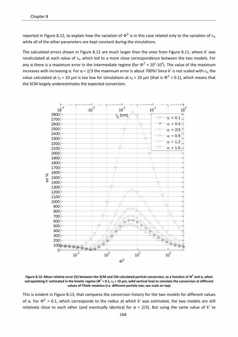
Chapter 8
164
reported in Figure 8.12, to explain how the variation of is in this case related only to the variation of r0,
while all of the other parameters are kept constant during the simulations.
The calculated errors shown in Figure 8.12 are much larger than the ones from Figure 8.11, where k’ was
recalculated at each value of r0, which led to a more close correspondence between the two models. For
any α there is a maximum error in the intermediate regime (for ≈ 101-102). The value of the maximum
increases with increasing α. For α = 2/3 the maximum error is about 700%! Since k’ is not scaled with r0, the
value calculated at r0 = 10 μm is too low for simulations at r0 > 10 μm (that is > 0.1), which means that
the SCM largely underestimates the expected conversion.
Figure 8.12: Mean relative error (%) between the SCM and CM calculated particle conversion, as a function of Ф2 and α, when
extrapolating k’ estimated in the kinetic regime (Ф2 = 0.1, r0 = 10 μm, solid vertical line) to simulate the conversion at different
values of Thiele modulus (i.e. different particle size; see scale on top)
This is evident in Figure 8.13, that compares the conversion history for the two models for different values
of α. For = 0.1, which corresponds to the radius at which k’ was estimated, the two models are still
relatively close to each other (and eventually identical for α = 2/3). But using the same value of k’ to
10-2
100
102
104
0
100
200
300
400
500
600
700
800
900
1000
1100
1200
1300
1400
1500
1600
1700
1800
1900
2000
2100
2200
2300
2400
2500
2600
2700
2800
2
err
%
= 0.1
= 0.4
= 2/3
= 0.9
= 1.2
= 1.6
10-4
10-3
10-2
10-1
100
r0 (cm)
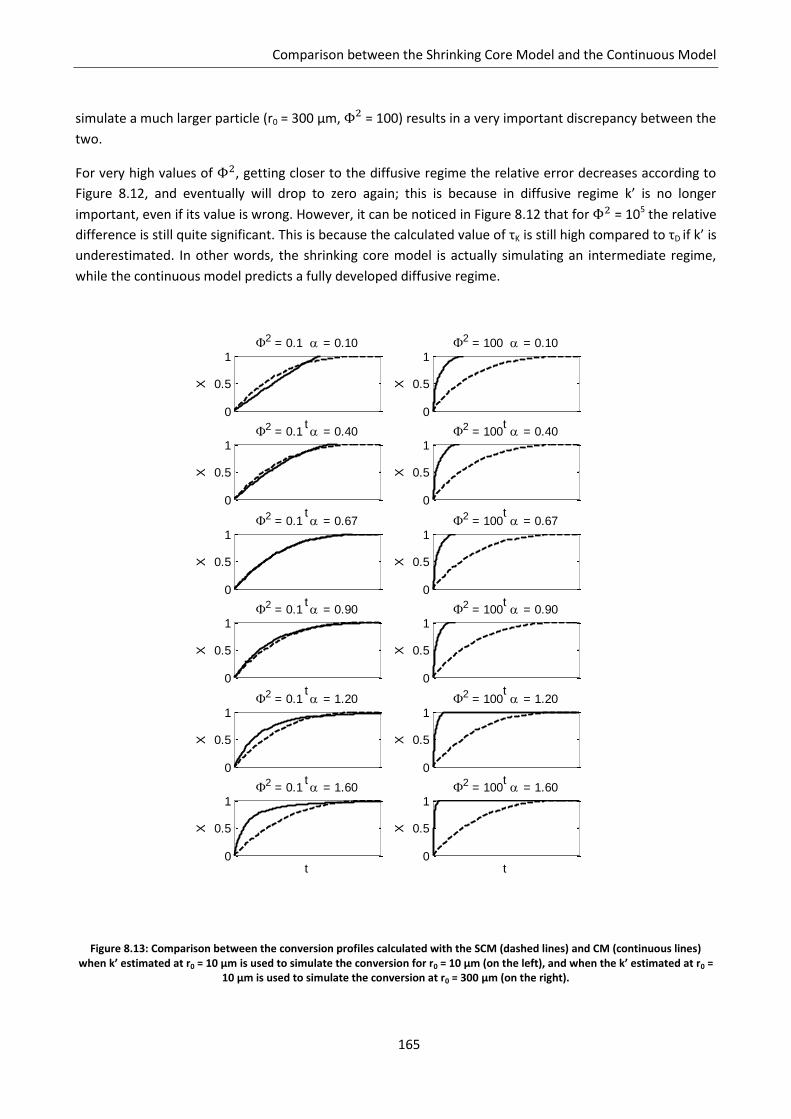
Comparison between the Shrinking Core Model and the Continuous Model
165
simulate a much larger particle (r0 = 300 μm, = 100) results in a very important discrepancy between the
two.
For very high values of , getting closer to the diffusive regime the relative error decreases according to
Figure 8.12, and eventually will drop to zero again; this is because in diffusive regime k’ is no longer
important, even if its value is wrong. However, it can be noticed in Figure 8.12 that for = 105 the relative
difference is still quite significant. This is because the calculated value of τK is still high compared to τD if k’ is
underestimated. In other words, the shrinking core model is actually simulating an intermediate regime,
while the continuous model predicts a fully developed diffusive regime.
Figure 8.13: Comparison between the conversion profiles calculated with the SCM (dashed lines) and CM (continuous lines) when k’ estimated at r0 = 10 μm is used to simulate the conversion for r0 = 10 μm (on the left), and when the k’ estimated at r0 =
10 μm is used to simulate the conversion at r0 = 300 μm (on the right).
0
0.5
12 = 0.1 = 0.10
t
X
0
0.5
12 = 100 = 0.10
t
X
0
0.5
12 = 0.1 = 0.40
t
X
0
0.5
12 = 100 = 0.40
t
X
0
0.5
12 = 0.1 = 0.67
t
X
0
0.5
12 = 100 = 0.67
t
X
0
0.5
12 = 0.1 = 0.90
t
X
0
0.5
12 = 100 = 0.90
t
X
0
0.5
12 = 0.1 = 1.20
t
X
0
0.5
12 = 100 = 1.20
t
X
0
0.5
12 = 0.1 = 1.60
t
X
0
0.5
12 = 100 = 1.60
t
X
Chapter 8
166
For < 0.1 (r0 < 10 μm), the value of k’ fitted for r0 = 10 μm is too high, and so the gap between the
models increases again, even if both models are simulating a kinetic regime. For α = 2/3, at = 0.001 (i.e.
r0 = 1 μm) the error is about 90%. This is only apparently in contrast with what was previously stated: in
kinetic regime, the SCM and CM become identical for α = 2/3 only if k’ is calculated for the same value of r0
used for the simulations, otherwise large differences may arise even in this case.
It can be noticed that, for α ≠ 2/3, the minimum of the error in kinetic regime is not reached for = 0.1.
This may seem odd, but it’s actually due to the fact that in our case the calculation of the optimum k’ was
made by minimizing the absolute difference, while the plot in Figure 8.12 shows the relative difference. By
default, at low conversions the SCM overestimates the CM for α<2/3 and underestimates it for α>2/3 (see
Figure 8.10). So if k’ is lower than k’opt, at α<2/3 the SCM will be more accurate at low conversions, which
results in a lower value of the integral mean of the relative error. The opposite happens for α>2/3 if k’>k’opt.
8.4 Conclusion
A comparison between the shrinking core model and the generalized grain model has been made. A
simplified version of the continuous model was considered (Fickian diffusion, no natural convection of the
gas, negligible effect of the variation of porosity), as well as a simple kinetics (a single irreversible reaction).
The study was focused on two aspects: the controlling regime, and the value of α, which is physically
related to the shape of the micro grains and the effect of sintering. For spherical grains (α = 2/3), the SCM
can well approximate the continuous model, and the global pellet conversion profiles are mathematically
equivalent in both kinetic and diffusive regime. The SCM does not represent the results of the CM if α ≠
2/3, except in the full diffusion control.
The discrepancy between the two models was evaluated for different sintering behavior (values of α) and
controlling regime (values of the Thiele modulus), after calculating the optimum value of the kinetic
constant for the SCM to fit the conversion profile from the continuous model.
Finally, since outside of the diffusive regime the SCM incorrectly describes the physics of the evolution of
the particle, it was proven that the value of the kinetic constant that fit the experimental data is not an
intrinsic parameter, but is affected by the size of the particle itself. For this reason, it must be pointed out
that the shrinking core model should be used very carefully, particularly when extrapolating the results at
different conditions from those of the experimental data used to fit the kinetics. If k’ was found in kinetic
regime, it should be wise to linearly scale it with the particle size in order to avoid severe errors.
Finally, due to the simplifications introduced for the CM, the errors of approximation of SCM to CM shown
by our work are quantified in the most optimistic situation, and in some cases they could be larger, if SCM
is compared with a more detailed version of CM. Despite this, the calculations reported allow concluding
that the classical assumption that SCM is a reasonable approximation of the reaction in any porous solids
could be dramatically wrong under several circumstances. The reported results will hopefully help the
practitioners to identify the most critical conditions in which the SCM leads to larger errors in simulating full
scale reactors involving reacting porous solids, well beyond the intrinsic limitations of the SCM as a model.
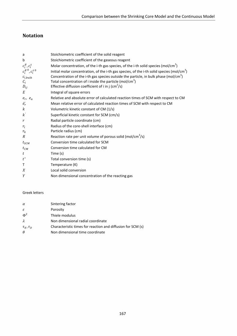
Comparison between the Shrinking Core Model and the Continuous Model
167
Notation
a Stoichiometric coefficient of the solid reagent
b Stoichiometric coefficient of the gaseous reagent
Molar concentration, of the i-th gas species, of the i-th solid species (mol/cm3)
Initial molar concentration, of the i-th gas species, of the i-th solid species (mol/cm
3)
Concentration of the i-th gas species outside the particle, in bulk phase (mol/cm3)
Total concentration of i inside the particle (mol/cm3)
Effective diffusion coefficient of i in j (cm2/s)
Integral of square errors
Relative and absolute error of calculated reaction times of SCM with respect to CM
Mean relative error of calculated reaction times of SCM with respect to CM
Volumetric kinetic constant of CM (1/s)
Superficial kinetic constant for SCM (cm/s)
Radial particle coordinate (cm)
Radius of the core-shell interface (cm) Particle radius (cm)
Reaction rate per unit volume of porous solid (mol/cm3/s)
Conversion time calculated for SCM
Conversion time calculated for CM
Time (s)
Total conversion time (s)
T Temperature (K)
Local solid conversion
Non dimensional concentration of the reacting gas
Greek letters
Sintering factor
Porosity
Thiele modulus
Non dimensional radial coordinate
Characteristic times for reaction and diffusion for SCM (s)
Non dimensional time coordinate

168
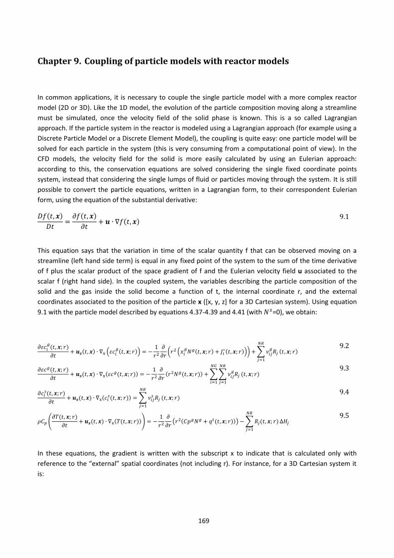
169
Chapter 9. Coupling of particle models with reactor models
In common applications, it is necessary to couple the single particle model with a more complex reactor
model (2D or 3D). Like the 1D model, the evolution of the particle composition moving along a streamline
must be simulated, once the velocity field of the solid phase is known. This is a so called Lagrangian
approach. If the particle system in the reactor is modeled using a Lagrangian approach (for example using a
Discrete Particle Model or a Discrete Element Model), the coupling is quite easy: one particle model will be
solved for each particle in the system (this is very consuming from a computational point of view). In the
CFD models, the velocity field for the solid is more easily calculated by using an Eulerian approach:
according to this, the conservation equations are solved considering the single fixed coordinate points
system, instead that considering the single lumps of fluid or particles moving through the system. It is still
possible to convert the particle equations, written in a Lagrangian form, to their correspondent Eulerian
form, using the equation of the substantial derivative:
9.1
This equation says that the variation in time of the scalar quantity f that can be observed moving on a
streamline (left hand side term) is equal in any fixed point of the system to the sum of the time derivative
of f plus the scalar product of the space gradient of f and the Eulerian velocity field u associated to the
scalar f (right hand side). In the coupled system, the variables describing the particle composition of the
solid and the gas inside the solid become a function of t, the internal coordinate r, and the external
coordinates associated to the position of the particle x ([x, y, z] for a 3D Cartesian system). Using equation
9.1 with the particle model described by equations 4.37-4.39 and 4.41 (with =0), we obtain:
9.2
9.3
9.4
9.5
In these equations, the gradient is written with the subscript x to indicate that is calculated only with
reference to the “external” spatial coordinates (not including r). For instance, for a 3D Cartesian system it
is:
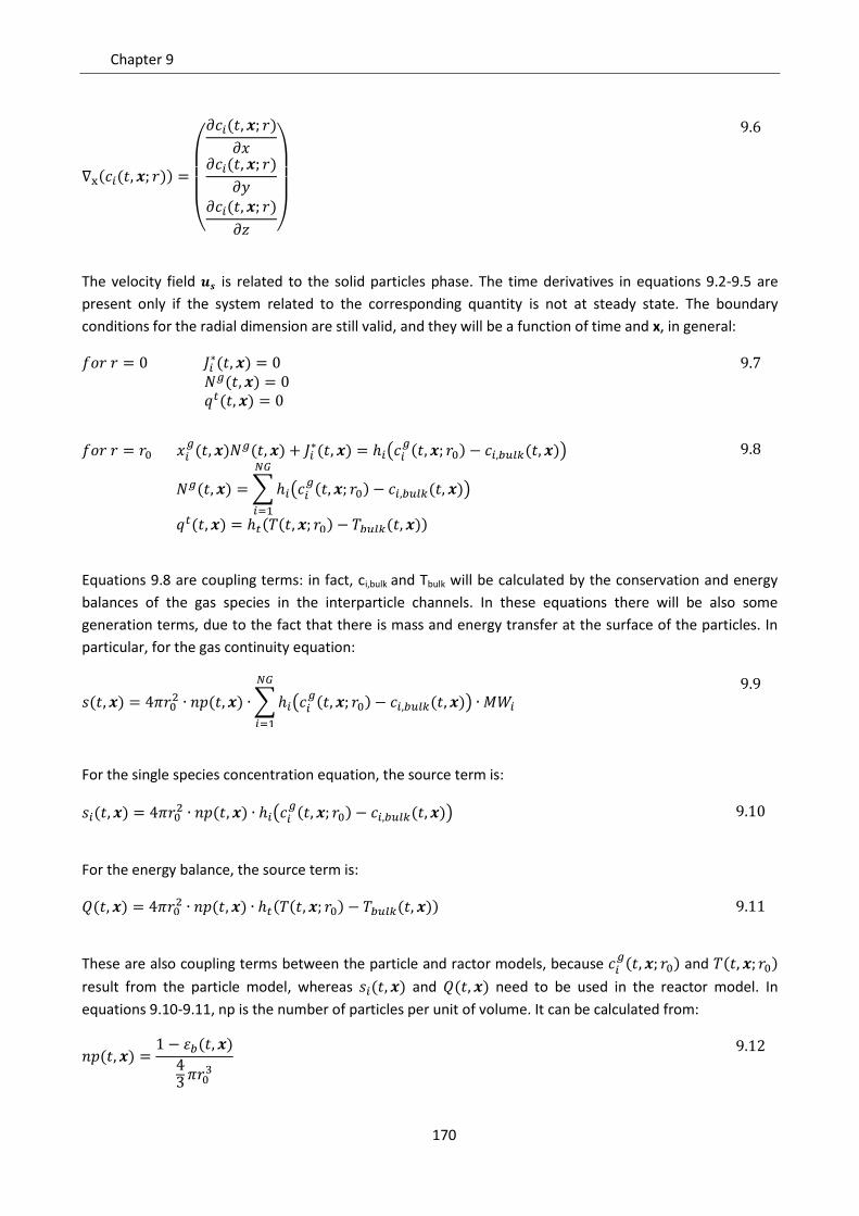
Chapter 9
170
9.6
The velocity field is related to the solid particles phase. The time derivatives in equations 9.2-9.5 are
present only if the system related to the corresponding quantity is not at steady state. The boundary
conditions for the radial dimension are still valid, and they will be a function of time and x, in general:
9.7
9.8
Equations 9.8 are coupling terms: in fact, ci,bulk and Tbulk will be calculated by the conservation and energy
balances of the gas species in the interparticle channels. In these equations there will be also some
generation terms, due to the fact that there is mass and energy transfer at the surface of the particles. In
particular, for the gas continuity equation:
9.9
For the single species concentration equation, the source term is:
9.10
For the energy balance, the source term is:
9.11
These are also coupling terms between the particle and ractor models, because and
result from the particle model, whereas and need to be used in the reactor model. In
equations 9.10-9.11, np is the number of particles per unit of volume. It can be calculated from:
9.12
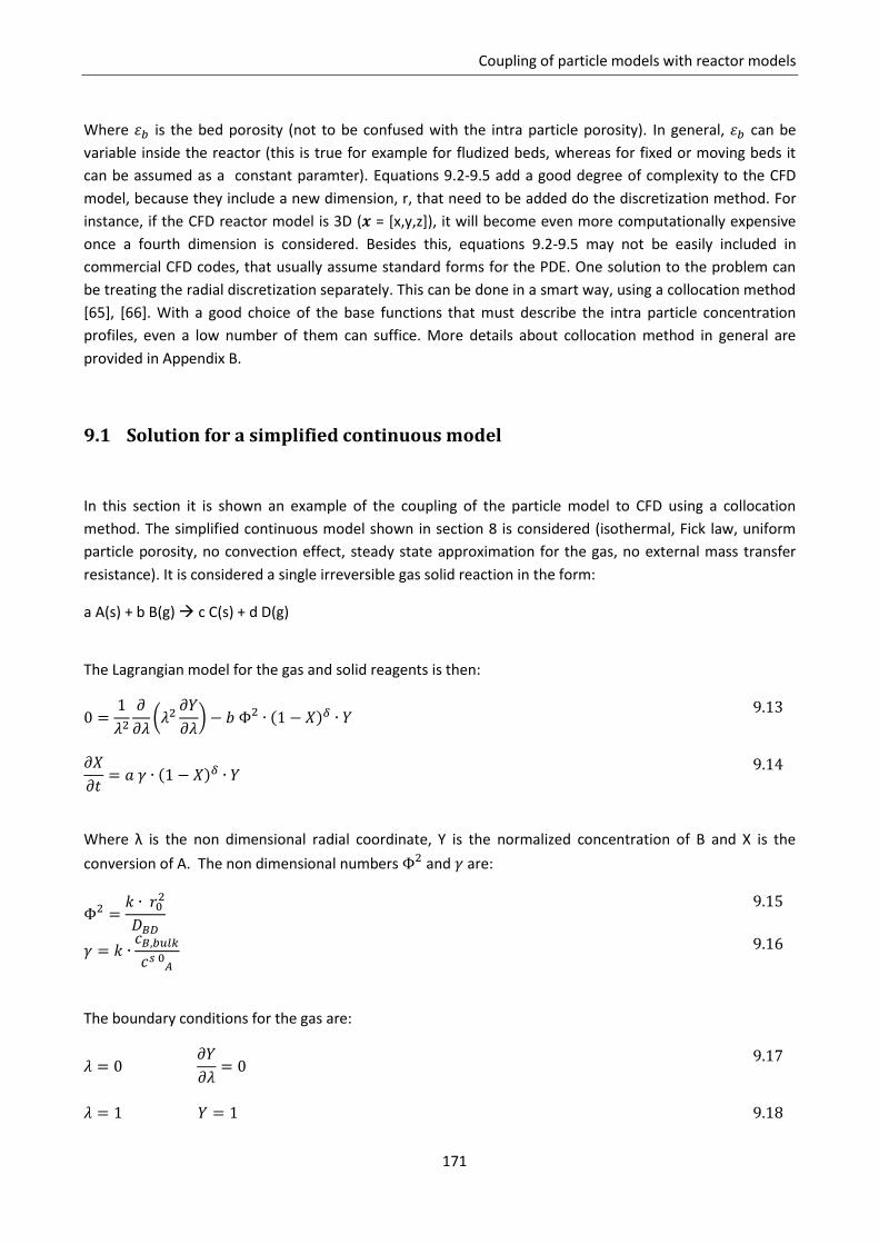
Coupling of particle models with reactor models
171
Where is the bed porosity (not to be confused with the intra particle porosity). In general, can be
variable inside the reactor (this is true for example for fludized beds, whereas for fixed or moving beds it
can be assumed as a constant paramter). Equations 9.2-9.5 add a good degree of complexity to the CFD
model, because they include a new dimension, r, that need to be added do the discretization method. For
instance, if the CFD reactor model is 3D ( = [x,y,z]), it will become even more computationally expensive
once a fourth dimension is considered. Besides this, equations 9.2-9.5 may not be easily included in
commercial CFD codes, that usually assume standard forms for the PDE. One solution to the problem can
be treating the radial discretization separately. This can be done in a smart way, using a collocation method
[65], [66]. With a good choice of the base functions that must describe the intra particle concentration
profiles, even a low number of them can suffice. More details about collocation method in general are
provided in Appendix B.
9.1 Solution for a simplified continuous model
In this section it is shown an example of the coupling of the particle model to CFD using a collocation
method. The simplified continuous model shown in section 8 is considered (isothermal, Fick law, uniform
particle porosity, no convection effect, steady state approximation for the gas, no external mass transfer
resistance). It is considered a single irreversible gas solid reaction in the form:
a A(s) + b B(g) c C(s) + d D(g)
The Lagrangian model for the gas and solid reagents is then:
9.13
9.14
Where λ is the non dimensional radial coordinate, Y is the normalized concentration of B and X is the
conversion of A. The non dimensional numbers and are:
9.15
9.16
The boundary conditions for the gas are:
9.17
9.18
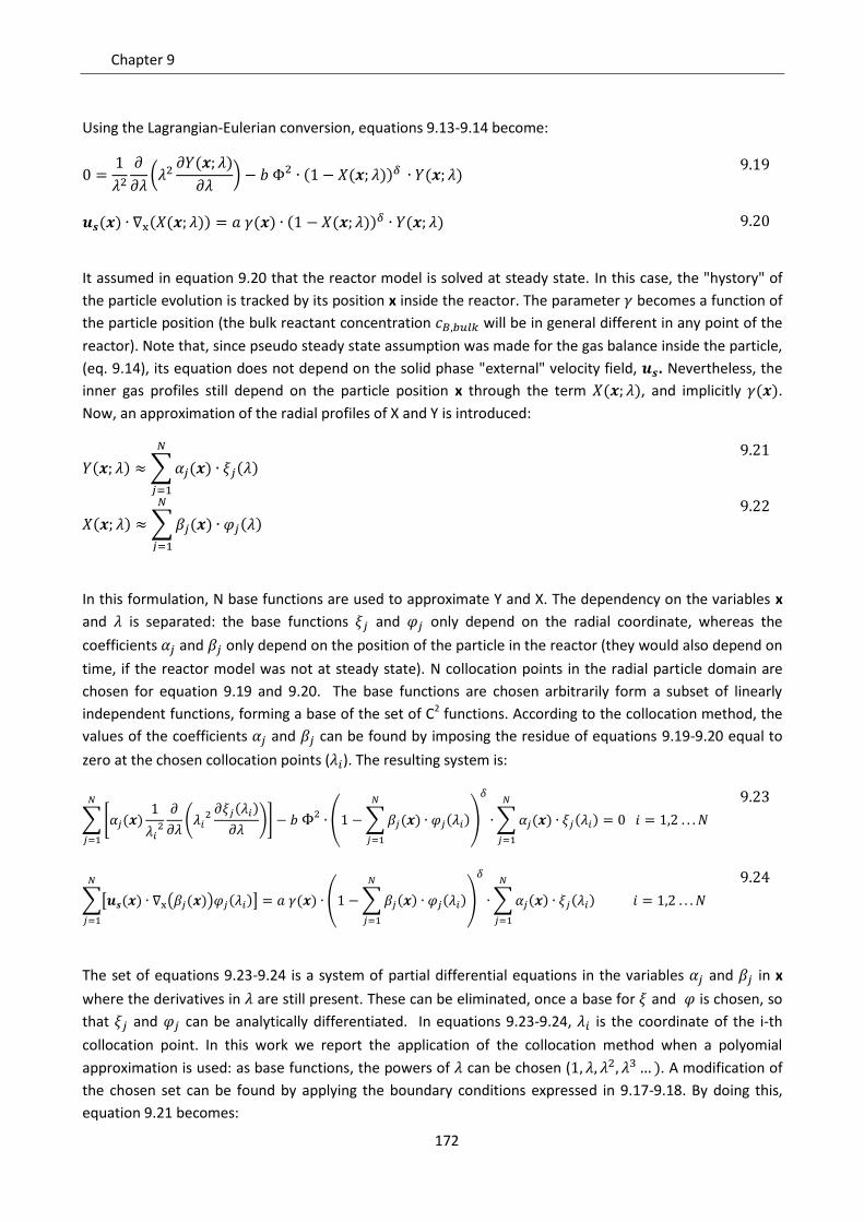
Chapter 9
172
Using the Lagrangian-Eulerian conversion, equations 9.13-9.14 become:
9.19
9.20
It assumed in equation 9.20 that the reactor model is solved at steady state. In this case, the "hystory" of
the particle evolution is tracked by its position x inside the reactor. The parameter becomes a function of
the particle position (the bulk reactant concentration will be in general different in any point of the
reactor). Note that, since pseudo steady state assumption was made for the gas balance inside the particle,
(eq. 9.14), its equation does not depend on the solid phase "external" velocity field, . Nevertheless, the
inner gas profiles still depend on the particle position x through the term , and implicitly .
Now, an approximation of the radial profiles of X and Y is introduced:
9.21
9.22
In this formulation, N base functions are used to approximate Y and X. The dependency on the variables x
and is separated: the base functions and only depend on the radial coordinate, whereas the
coefficients and only depend on the position of the particle in the reactor (they would also depend on
time, if the reactor model was not at steady state). N collocation points in the radial particle domain are
chosen for equation 9.19 and 9.20. The base functions are chosen arbitrarily form a subset of linearly
independent functions, forming a base of the set of C2 functions. According to the collocation method, the
values of the coefficients and can be found by imposing the residue of equations 9.19-9.20 equal to
zero at the chosen collocation points ( ). The resulting system is:
9.23
9.24
The set of equations 9.23-9.24 is a system of partial differential equations in the variables and in x
where the derivatives in are still present. These can be eliminated, once a base for and is chosen, so
that and can be analytically differentiated. In equations 9.23-9.24, is the coordinate of the i-th
collocation point. In this work we report the application of the collocation method when a polyomial
approximation is used: as base functions, the powers of can be chosen ( . A modification of
the chosen set can be found by applying the boundary conditions expressed in 9.17-9.18. By doing this,
equation 9.21 becomes:
Coupling of particle models with reactor models
173
9.25
The approximation of the first derivative of Y in becomes:
9.26
It is trivial to prove that the boundary conditions are always verified for any value of the set of coefficients
. Note that by doing this, the first order monomer is automatically excluded from the approximation of
Y. This is coherent with the fact that the solution of the equation must be searched within a subspace of
continuous and twice derivable functions that respect the boundary conditions, and for this reason some
constraints are applied to the set of base functions. For the solution of the solid, X, no boundary conditions
need to be imposed by the problem. Yet, a “natural“ condition on the shape of the solution derives from
the symmetry at . So it is wise to choose a set of base functions for X so that the approximation of X is
smooth at . For instance:
9.27
Applying equations 9.25-9.27 to the collocation formulation, equations 9.23-9.24 become:
9.28
9.29
The resulting equations are non linear, so the source term has to be linearized and then the system can be
solved iteratively. According to a Newton-Raphson scheme, the reaction term in equations 9.19-9.20 can be
calculated at the n+1 iteration as follows:
9.30
The equations to solve, in the variables and , become in a matrix form:
Chapter 9
174
9.31
9.32
The matrices A, B, A’’, ,
and the vector are defined from equations 9.33-9.38, whereas I is the
identity matrix:
9.33
9.34
9.35
9.36
9.37
9.38
Note that A, B, A’’ are constant, so they can be calculated once the number and position of the collocation
points are chosen. On the contrary, ,
and depend on the values of the variables calculated at the
previous iteration. Equation 9.31 is linear algebraic, while 9.32 is differential with respect to the variables x.
They must be solved iteratively until convergence (this will imply that equation 9.32 must be integrated and
equation 9.31 must be solved using the matrices calculated at the n-th iteration, until the solution at n+1 is
equal to the solution at n). The gradient is defined as:
9.39
Once the solution in and is obtained, the mean particle solid conversion can be found in any
point of the reactor by calculating the following integral:
9.40
The source term for the bulk gas composition for the reactant B becomes:
Coupling of particle models with reactor models
175
9.41
The computational cost added to the problem with the particle model is strictly related to the chosen
number of collocation points. For the considered simplified particle model and reaction mechanism, one
PDE and one algebraic equation are added to the problem for every collocation point. Few collocation
points can also mean a low accuracy in the approximation of the intra particle profiles, and high errors in
the solution. An optimum value must be chosen, depending on the problem to solve. It is also important to
point out that, for a fixed number of collocation points, the accuracy of the approximated solution can
easily depend on the form of the base functions (in this example, polynomials were used). If the analytical
shapes of the base functions are more similar to the real solution profile, it is more likely that a low number
of them can suffice to obtain a good result. This "efficiency" cannot be evaluated a priori, but depends on
the considered problem, and specific numerical tests are needed to identify the best choice.
9.2 Coupling with 1D moving bed reactor model
The mathematical approach described by equations 9.2-9.5 can be easily applied to a one dimension
reactor model. In this section the example of a moving bed reactor is considered. The reactor is assumed to
be cylindrical, with a stream of reacting gas flowing from the bottom to the top. At the same time, a
counter current flow rate of solid particles is fed at the top of the reactor. The reacting gas flows in the
spaces between the particles, and diffuses inside them converting the solid species. If all the characteristics
of the solid and gas phases are assumed to be uniform along the reactor radial coordinate, a one dimension
reactor model can be used.
The solid particles are supposed to flow along the axial coordinate along parallel streamlines at a constant
velocity. The entire reactor works at steady state. If these assumptions are correct, the particle model
expressed by equations 9.2-9.5 becomes:
9.42
9.43
9.44
9.45
Equations 9.42-9.45 are the equations for the concentration of gas species, total gas concentration,
concentration of solid species and energy inside the particle, respectively. In this formulation, is a
Chapter 9
176
parameter. The boundary conditions for the gas inside the particle are the same reported by equations 9.7-
9.8. The gas species concentration balances in the channels between particles are in the form:
9.46
Equation 9.46 considers convection, diffusion and a source term due to the mass transfer of the gas i from
the bulk to the particles or vice versa. The source term is again expressed through equation 9.10, i.e. the
species flux of the i-th species from the particle external surface to the gas, as given by the particle model.
A total concentration balance must be added to evaluate the axial gas velocity profile:
9.47
The energy balance for the bulk gas phase is:
9.48
Where the source term Q is expressed through equation 9.11, i.e. the heat flux from the particle external
surface to the gas, as given by the particle model. Boundary conditions bust be also added at the reactor
gas inlet and solid inlet. Assuming that z = 0 is the solid inlet and the gas outlet, and z = L is the gas inlet and
solid outlet, the boundary conditions are:
9.49
9.50
The numerical treatment of the problem expressed by equations 9.42-9.48 is relatively simple. Once a
discretization scheme is applied to the radial particle dimension in equations 9.42-9.45, the resulting
system is only made of ordinary differential equations in z. The only further difficulty is related to the fact
that the boundary conditions are both at z = 0 and z = L, so the system cannot be treated as an initial value
problem but as a boundary value problem.
Figure 9.1 shows an example of solution obtained for the moving bed reactor model, for an isothermal case
(equations 9.42-9.44 and 9.46-9.47). The model has been implemented in Matlab [23], using a finite
volume method to express the radial derivative and then using a BVP solver to solve the resulting ODE
system. The reaction mechanism considered is the reduction of Hematite to Metallic Iron with CO, in three
steps:
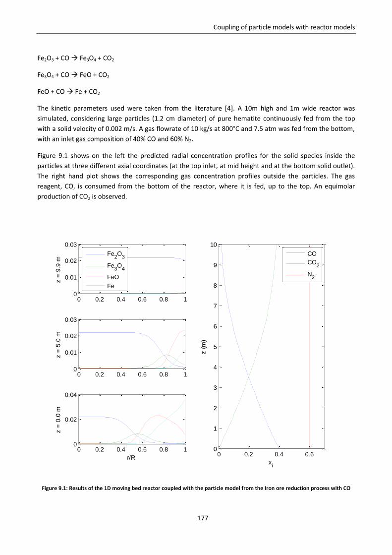
Coupling of particle models with reactor models
177
Fe2O3 + CO Fe3O4 + CO2
Fe3O4 + CO FeO + CO2
FeO + CO Fe + CO2
The kinetic parameters used were taken from the literature [4]. A 10m high and 1m wide reactor was
simulated, considering large particles (1.2 cm diameter) of pure hematite continuously fed from the top
with a solid velocity of 0.002 m/s. A gas flowrate of 10 kg/s at 800°C and 7.5 atm was fed from the bottom,
with an inlet gas composition of 40% CO and 60% N2.
Figure 9.1 shows on the left the predicted radial concentration profiles for the solid species inside the
particles at three different axial coordinates (at the top inlet, at mid height and at the bottom solid outlet).
The right hand plot shows the corresponding gas concentration profiles outside the particles. The gas
reagent, CO, is consumed from the bottom of the reactor, where it is fed, up to the top. An equimolar
production of CO2 is observed.
Figure 9.1: Results of the 1D moving bed reactor coupled with the particle model from the Iron ore reduction process with CO
0 0.2 0.4 0.60
1
2
3
4
5
6
7
8
9
10
xi
z (
m)
CO
CO2
N2
0 0.2 0.4 0.6 0.8 10
0.01
0.02
0.03
z =
9.9
m
Fe2O
3
Fe3O
4
FeO
Fe
0 0.2 0.4 0.6 0.8 10
0.01
0.02
0.03
z =
5.0
m
0 0.2 0.4 0.6 0.8 10
0.02
0.04
z =
0.0
m
r/R
Chapter 9
178
Notation
Molar concentration, of the i-th gas species, of the i-th solid species (mol/cm3)
Initial molar concentration, of the i-th gas species, of the i-th solid species (mol/cm
3)
Concentration of the i-th solid species at the particles inlet (mol/cm
3)
Total concentration of gas phase, of solid phase (mol/cm3)
Concentration of the i-th gas species outside the particle, in bulk phase (mol/cm3)
Concentration of the i-th gas species in bulk phase, at the gas reactor inlet (mol/cm
3)
Heat capacity of the medium (J/cm3/K)
Heat capacity of the gas phase, of the solid phase (J/mol/K) Effective diffusion coefficient of i in j (cm
2/s)
Mass transfer coefficient of i (cm/s) Heat transfer coefficient (W/cm
2/K)
Molar diffusive flux of i (mol/cm
2/s)
Volumetric kinetic constant of CM (1/s)
Molecular weight of the i-th species (g/mol) Number of particles per unit of reactor volume (1/cm
3)
Number of base functions Total molar flux of the gas phase (mol/cm
2/s)
Number of gas species in the system Number of reactions Number of solid species in the system Conductive flux (W/cm
2)
Source term for the energy balance for the gas in bulk phase (W/cm3)
Radial particle coordinate (cm)
Particle radius (cm)
Source term for the continuity equation of the gas bulk phase (g/cm3/s)
Source term for the concentration balance of the i-th gas in bulk phase (mol/cm3/s)
Rate of the i-th reaction (mol/cm3/s)
Time (s) Absolute temperature, local, outside the particle in bulk phase (K)
Absolute temperature of gas in bulk phase at the gas reactor inlet (K)
Velocity of the gas in bulk phase (cm/s)
Velocity of the gas in bulk phase at the gas reactor inlet (cm/s)
Velocity field of the solid particles medium (cm/s) Vector of spatial coordinates (cm) i-th spatial coordinate in the reactor reference system
, Molar fraction of the i-th gas species, of the i-th solid species
Local solid conversion
Mean particle conversion
Non dimensional concentration of the reacting gas
Greek letters
Coefficient of the i-th base function approximating Y
Coefficient of the i-th base function approximating X
Sintering factor
Heat of the j-th reaction, molar based (J/mol)
Particle porosity
Bed porosity

Coupling of particle models with reactor models
179
Thiele modulus
Non dimensional radial coordinate
Coordinate of the i-th collocation point
Stoichiometric coefficient of the i-th gas species in the j-th reaction
Stoichiometric coefficient of the i-th solid species in the j-th reaction
i-th base function approximating Y i-th base function approximating X

Chapter 9
180
181
Chapter 10. Conclusions
The aim of this thesis was to evaluate the reliability of the different approaches that can be used while
modeling non catalytic gas-solid reactions, with particular interest in single particle models. This study was
carried out both by theoretical analyses of the models results, and by comparison with experimental data
from different processes. The final goal was to understand the importance of using detailed continuous
models, instead of the simpler core-shell reaction rate.
The first base case considered was the application of the Shrinking Core Model to the reduction of hematite
to metallic iron with syngas. A CFD model was developed to simulate the process in shaft furnaces, with a
flux of reacting spherical particles in countercurrent with a stream of gas at high temperature and pressure.
The model allowed solving the velocity fields, compositions and temperatures of both solid and gas phases.
After a fitting of the kinetic parameters of SCM to experimental data, the model was able to predict the
solid conversions of the two phases both in the full scale plants and in the pilot plants, that were realized
within the industrial project to study the particle reaction rates. The simulated particles in this process are
quite large (about 2 cm diameter), which results in an important contribution of the diffusion resistance in
the overall mechanism of particle conversion: this is the situation when a core-shell structure is really
formed, and the SCM is able to correctly describe the heterogeneous process. This explains the good
predictivity of the model, in comparison with the available evidences. The choice of SCM in the simulation
of industrial processes is often dictated by its straightforward applicability to CFD, yet it is sometimes
proven to work because it can still consider both kinetic and intra particle diffusion phenomena.
A good agreement with the experimental data is not always a guarantee that the model is good per se. As a
matter of fact, the data regression can dissimulate the incorrect or approximated description of mass
transport phenomena, by discharging these errors into the quantification of the unknown parameters. For
this reason, an analysis of more detailed particle models (continuous models) was performed.
The sensitivity tests on the accuracy of the diffusion model proved that the use of a rigorous Stefan-
Maxwell approach can be necessary in most of the cases where intraparticle diffusion is important. This is
particularly true when the concentration of gas reagent into the mixture is high. The simplified mixture
averaged model, with an effective coefficient calculated on the composition of the mixture is proved to be
a very good alternative, with resulting errors that are quite low (below 5%) even for heterogeneous gas
mixtures with species with very different diffusivities. On the contrary, the binary Fick’s Law with a constant
diffusion coefficient can lead to severe discrepancies in the prediction of the global particle conversion for
high Thiele modulus (also 10-50% for the most difficult cases). This issue should be really taken into
consideration, because it is common practice to simplify the form of the diffusion fluxes to be used in the
continuous model, also to obtain a more direct and easy numerical implementation.
A detailed investigation was carried out on the role of natural convection as a mechanism of mass transport
into the porous matrix. This is in most cases neglected in the literature, because diffusion is assumed to be
largely dominant. In our analysis, three different sources of natural convection into the reacting particle
were identified: the effect of changing porosity (which reflects on the changing gas volume due to the
change of the molar density of the solid during the reaction), the effect of temperature gradients (and so
different density of the gas in different points of the particle), and the net production or consumption of
Chapter 10
182
number of gas moles related to the reaction stoichiometry. The first two contributions were proven to be
negligible, whereas it was shown that the presence of a non equimolar reaction in gas phase could imply
the inclusion of convection into the model for a more correct description of the process. Nevertheless, the
performed simulations for the considered examples showed limited errors in the determination of the
global particle conversion, when convection is not considered (maximum 5-8% for the non equimolar
reaction of oxidation of zinc sulphide).
The continuous model was applied to describe the reduction of metal oxides with syngas, considering solid
particles used as oxygen carriers for chemical looping combustion. Chemical looping is a classical example
of process where the evolution of the porous solid matrix due to physical and chemical phenomena is
expected to have a great influence on the reacting system, because of the high number of reaction cycles
involving the same particles. This is evident from experimental data that show an improvement of the solid
reactivity with increasing number of cycles. Another characteristic of the oxygen carriers reactivity is that it
greatly decreases for high conversions, and this is largely documented by TGA analyses. Different
hypotheses were made to try to describe the particle conversion profiles with the continuous model.
Namely, solid sintering, the effect of pore size distribution, the effect of gas diffusion in dense solid, and the
effect of solid phase segregation were considered. These phenomena were independently implemented
into different formulations of the particle model. All these versions were able to explain the TGA data,
except for the model including the experimental pore size distribution. This proved that, for the considered
example, the effect of different effective diffusivities in pores with different size cannot be responsible for a
change of the controlling regime during the particle conversion. On the other hand, the reactivity
slowdown could be either the result of one of the following phenomena:
- An important decrease of the superficial area of the reacting solid with time due to sintering of
micrograins at high temperature.
- The presence of fractions of solid matrix that are not reached by pores, where the diffusion
resistance of gas transportation plays an important role.
- The presence in activated particles of segregated solid phases with different reactivities, that
can lead to two kinetic steps (fast and slow reaction).
The first two results are just a consequence of preliminary assumptions, whereas the third one is confirmed
in the case of the ilmenite-pseudobrookite system by an experimental characterization of the solid
activated particles, that really shows the existence of different solid phases, and a slow process of their
redistribution within the core and an outer layer of the particle during the activation steps. The sensitivity
analysis made on the new implemented model also shows that a different reactivity of these solid phases
could explain both the conversion rate decrease of the particles during a single cycle, and the reactivity
increase with increasing number of cycles, due to the fact that the more reactive phase (hematite)
separates from the slow reacting one (pseudobrookite) in the first loops. This interpretation must be
further validated in the future, for the considered system. In particular, the results of the fitting of the
continuous model suggest that a different initial pseudobrookite degree of dissociation is required at
different temperatures to explain the experimental behavior, and this must be still demonstrated.
Two important conclusions can be made from the results of the work on chemical looping combustion:
first, it is quite easy that, for gas-solid reaction processes, the particle reactivity can be successfully
described only if a non trivial interaction phenomenon between the evolution of the solid morphology and
the process is considered and included into the particle model, and this cannot be done through the
Conclusions
183
shrinking core model, but a more detailed approach is necessary; second, the results show that an
experimental quantification of the global solid reactivity is surely necessary but not sufficient to fully
understand all the chemical-physical phenomena controlling the process. A thorough characterization of
the properties of the solid matrix, possibly obtained at several conversion steps, can be the key factor to
discriminate through different possible explanations of the same TGA profiles.
The importance of using a detailed approach was also assessed with the final comparison between the
Shrinking Core Model and a simplified version of the Continuous Model. The study was carried out by
considering different controlling regimes, and different forms of the gas-solid reaction rate used in the
continuous particle model. On the one hand, the results prove that the SCM can in several cases well
approximate the results of the CM, not only in diffusive regime as it is already stated in the literature, but
also for a kinetic controlled process, in the case of the grain model. A mathematical function was derived,
that relates the kinetic constant of the shrinking core model to that of the continuous model, that
minimizes the difference between the results of the two. On the other hand, the quantification of the
kinetic constant used in the shrinking core model was proved to be affected by the particle size. Very high
errors (> 100!) can arise if the SCM is used to simulate particles with very different sizes from those
corresponding to the conditions of the kinetic fitting. This highly limits the possibility of extrapolating the
results of the SCM in gas-solid simulations.
In conclusion, this thesis provides some insight into the modeling of gas-solid reaction problems, providing
some tools to more wisely evaluate the importance of several degrees of detail to be included when
choosing a single particle model.

Chapter 10
184
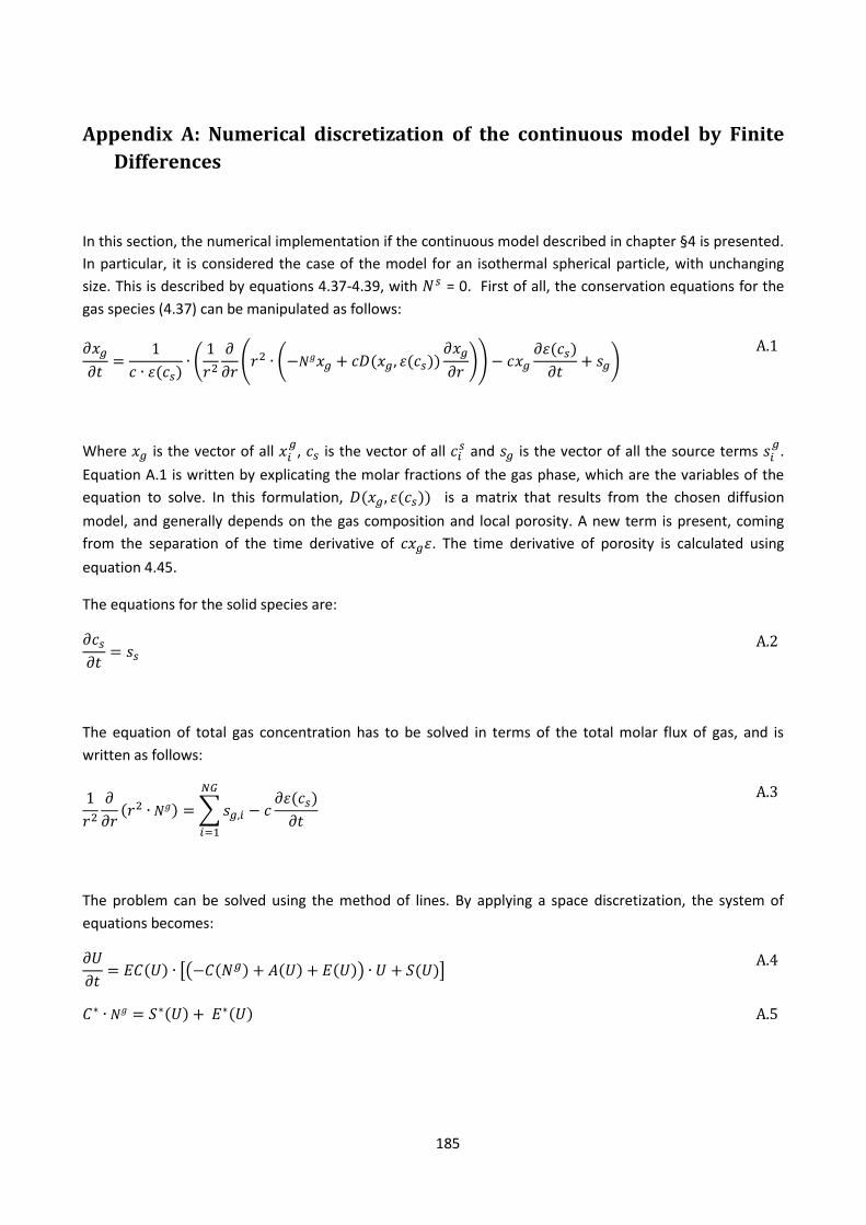
185
Appendix A: Numerical discretization of the continuous model by Finite
Differences
In this section, the numerical implementation if the continuous model described in chapter §4 is presented.
In particular, it is considered the case of the model for an isothermal spherical particle, with unchanging
size. This is described by equations 4.37-4.39, with = 0. First of all, the conservation equations for the
gas species (4.37) can be manipulated as follows:
A.1
Where is the vector of all
, is the vector of all and is the vector of all the source terms
.
Equation A.1 is written by explicating the molar fractions of the gas phase, which are the variables of the
equation to solve. In this formulation, is a matrix that results from the chosen diffusion
model, and generally depends on the gas composition and local porosity. A new term is present, coming
from the separation of the time derivative of . The time derivative of porosity is calculated using
equation 4.45.
The equations for the solid species are:
A.2
The equation of total gas concentration has to be solved in terms of the total molar flux of gas, and is
written as follows:
A.3
The problem can be solved using the method of lines. By applying a space discretization, the system of
equations becomes:
A.4
A.5
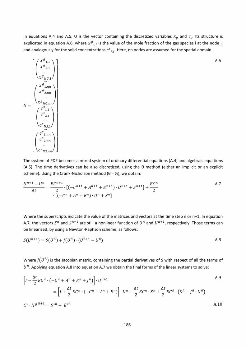
186
In equations A.4 and A.5, U is the vector containing the discretized variables and . Its structure is
explicated in equation A.6, where is the value of the mole fraction of the gas species i at the node j,
and analogously for the solid concentrations . Here, nn nodes are assumed for the spatial domain.
A.6
The system of PDE becomes a mixed system of ordinary differential equations (A.4) and algebraic equations
(A.5). The time derivatives can be also discretized, using the θ method (either an implicit or an explicit
scheme). Using the Crank-Nicholson method (θ = ½), we obtain:
A.7
Where the superscripts indicate the value of the matrices and vectors at the time step n or n+1. In equation
A.7, the vectors and are still a nonlinear function of and , respectively. Those terms can
be linearized, by using a Newton-Raphson scheme, as follows:
A.8
Where is the Jacobian matrix, containing the partial derivatives of S with respect of all the terms of
. Applying equation A.8 into equation A.7 we obtain the final forms of the linear systems to solve:
A.9
A.10
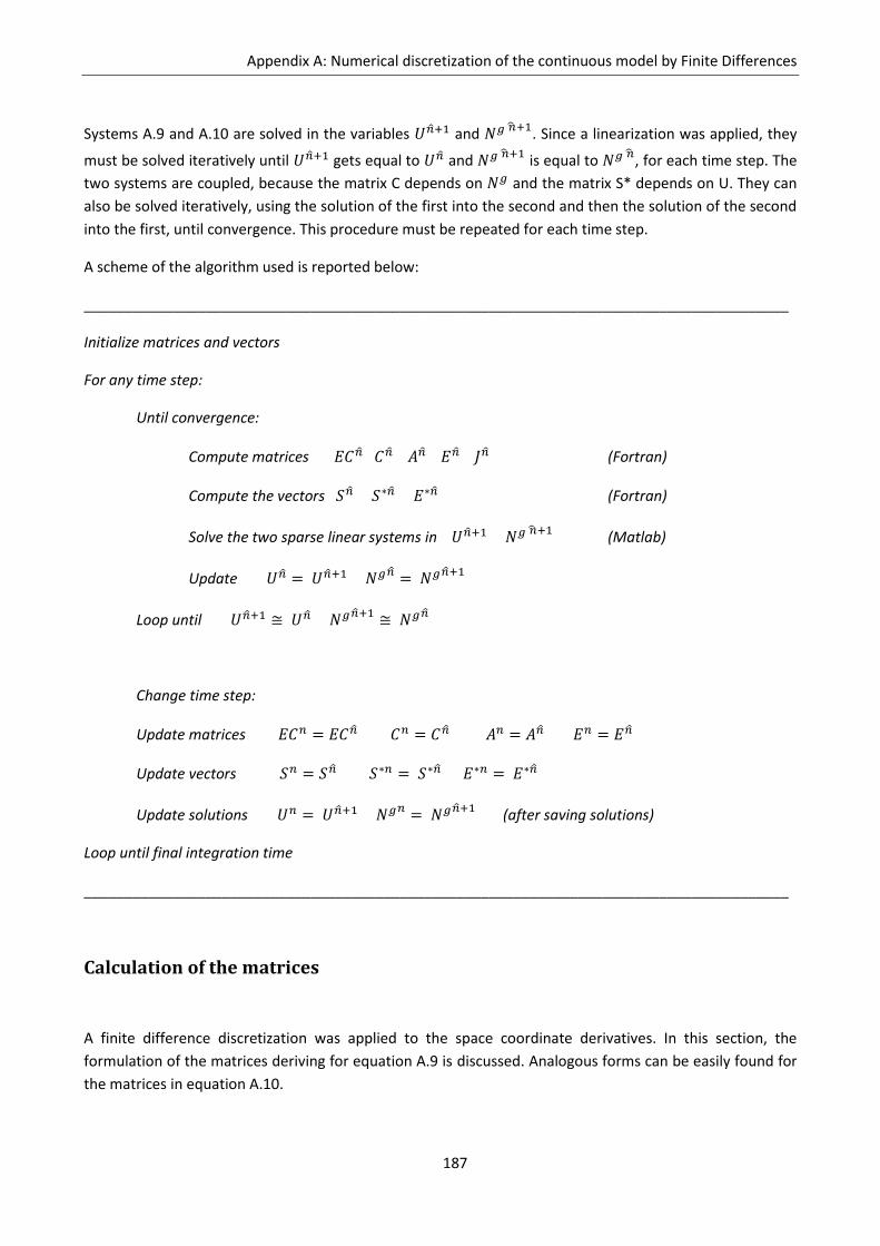
Appendix A: Numerical discretization of the continuous model by Finite Differences
187
Systems A.9 and A.10 are solved in the variables and . Since a linearization was applied, they
must be solved iteratively until gets equal to and is equal to
, for each time step. The
two systems are coupled, because the matrix C depends on and the matrix S* depends on U. They can
also be solved iteratively, using the solution of the first into the second and then the solution of the second
into the first, until convergence. This procedure must be repeated for each time step.
A scheme of the algorithm used is reported below:
_______________________________________________________________________________________
Initialize matrices and vectors
For any time step:
Until convergence:
Compute matrices (Fortran)
Compute the vectors (Fortran)
Solve the two sparse linear systems in (Matlab)
Update
Loop until
Change time step:
Update matrices
Update vectors
Update solutions (after saving solutions)
Loop until final integration time
_______________________________________________________________________________________
Calculation of the matrices
A finite difference discretization was applied to the space coordinate derivatives. In this section, the
formulation of the matrices deriving for equation A.9 is discussed. Analogous forms can be easily found for
the matrices in equation A.10.
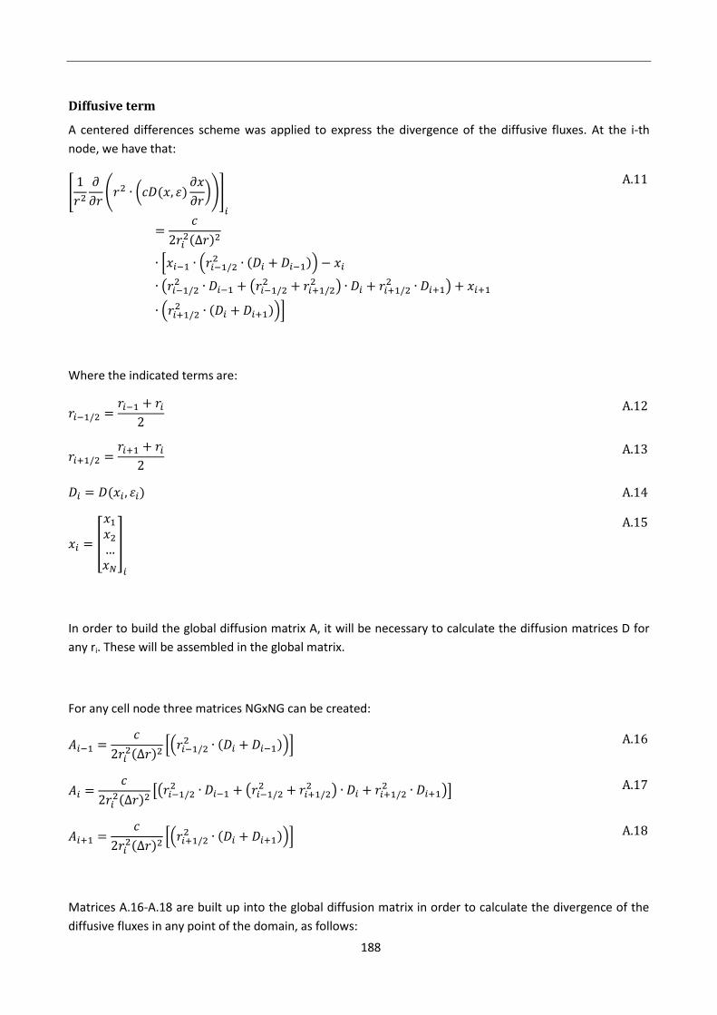
188
Diffusive term
A centered differences scheme was applied to express the divergence of the diffusive fluxes. At the i-th
node, we have that:
A.11
Where the indicated terms are:
A.12
A.13
A.14
A.15
In order to build the global diffusion matrix A, it will be necessary to calculate the diffusion matrices D for
any ri. These will be assembled in the global matrix.
For any cell node three matrices NGxNG can be created:
A.16
A.17
A.18
Matrices A.16-A.18 are built up into the global diffusion matrix in order to calculate the divergence of the
diffusive fluxes in any point of the domain, as follows:
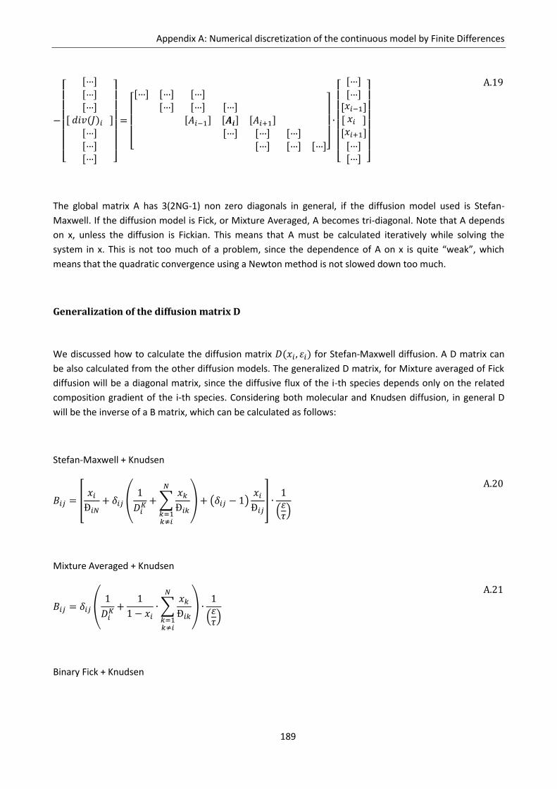
Appendix A: Numerical discretization of the continuous model by Finite Differences
189
A.19
The global matrix A has 3(2NG-1) non zero diagonals in general, if the diffusion model used is Stefan-
Maxwell. If the diffusion model is Fick, or Mixture Averaged, A becomes tri-diagonal. Note that A depends
on x, unless the diffusion is Fickian. This means that A must be calculated iteratively while solving the
system in x. This is not too much of a problem, since the dependence of A on x is quite “weak”, which
means that the quadratic convergence using a Newton method is not slowed down too much.
Generalization of the diffusion matrix D
We discussed how to calculate the diffusion matrix for Stefan-Maxwell diffusion. A D matrix can
be also calculated from the other diffusion models. The generalized D matrix, for Mixture averaged of Fick
diffusion will be a diagonal matrix, since the diffusive flux of the i-th species depends only on the related
composition gradient of the i-th species. Considering both molecular and Knudsen diffusion, in general D
will be the inverse of a B matrix, which can be calculated as follows:
Stefan-Maxwell + Knudsen
A.20
Mixture Averaged + Knudsen
A.21
Binary Fick + Knudsen
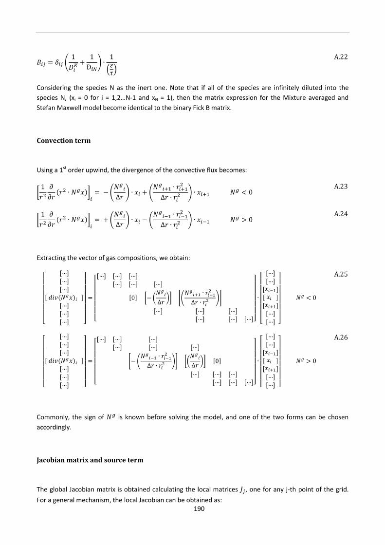
190
A.22
Considering the species N as the inert one. Note that if all of the species are infinitely diluted into the
species N, (xi = 0 for i = 1,2…N-1 and xN = 1), then the matrix expression for the Mixture averaged and
Stefan Maxwell model become identical to the binary Fick B matrix.
Convection term
Using a 1st order upwind, the divergence of the convective flux becomes:
A.23
A.24
Extracting the vector of gas compositions, we obtain:
A.25
A.26
Commonly, the sign of is known before solving the model, and one of the two forms can be chosen
accordingly.
Jacobian matrix and source term
The global Jacobian matrix is obtained calculating the local matrices , one for any j-th point of the grid.
For a general mechanism, the local Jacobian can be obtained as:
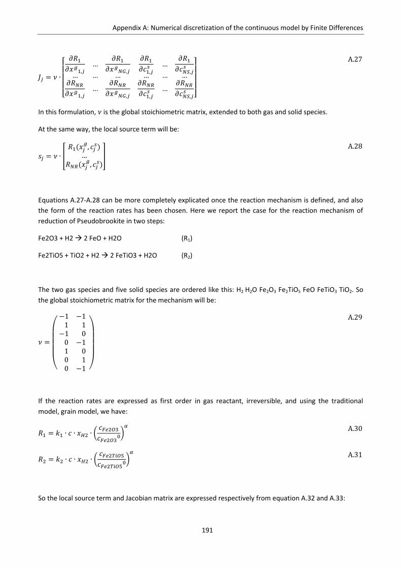
Appendix A: Numerical discretization of the continuous model by Finite Differences
191
A.27
In this formulation, is the global stoichiometric matrix, extended to both gas and solid species.
At the same way, the local source term will be:
A.28
Equations A.27-A.28 can be more completely explicated once the reaction mechanism is defined, and also
the form of the reaction rates has been chosen. Here we report the case for the reaction mechanism of
reduction of Pseudobrookite in two steps:
Fe2O3 + H2 2 FeO + H2O (R1)
Fe2TiO5 + TiO2 + H2 2 FeTiO3 + H2O (R2)
The two gas species and five solid species are ordered like this: H2 H2O Fe2O3 Fe2TiO5 FeO FeTiO3 TiO2. So
the global stoichiometric matrix for the mechanism will be:
A.29
If the reaction rates are expressed as first order in gas reactant, irreversible, and using the traditional
model, grain model, we have:
A.30
A.31
So the local source term and Jacobian matrix are expressed respectively from equation A.32 and A.33:
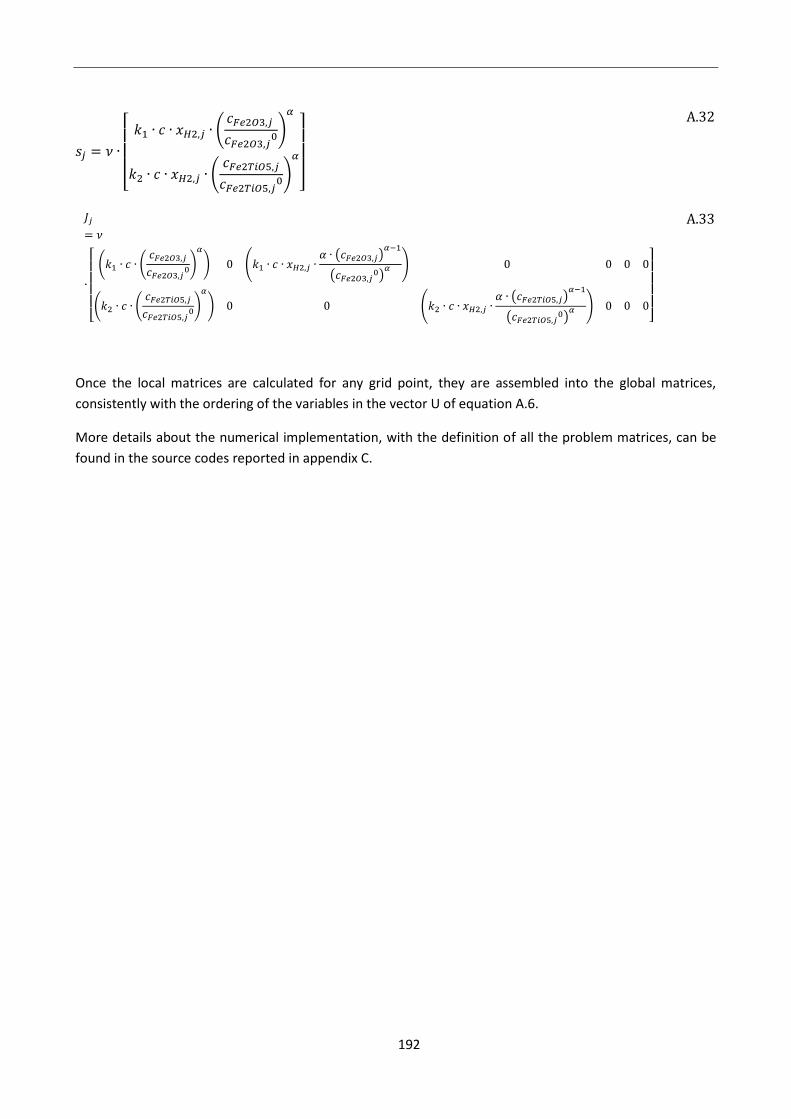
192
A.32
A.33
Once the local matrices are calculated for any grid point, they are assembled into the global matrices,
consistently with the ordering of the variables in the vector U of equation A.6.
More details about the numerical implementation, with the definition of all the problem matrices, can be
found in the source codes reported in appendix C.
193
Appendix B: Basics of Weighted Residual Methods
Let us consider a generic partial differential equation, and defined as follows:
D(u(x)) = f A.34
Where u(x) is the unknown function, defined in the domain Ω, D is a generic differential operator, and f is a
known function. An approximation ũ(x) of the exact solution can be defined, as a linear combination of N
continuous base functions , linearly independent from each other:
A.35
It can be mathematically proved that if N∞, there is a set of coefficients aj such that ũ = u. In practical
applications, a finite number of coefficients aj must be found, such that ũ approximates u as well as
possible. In order to define a criterion of “good approximation”, the residual R of ũ is defined, as a function
of the set of coefficients a = [a1, a2,… aN]:
A.36
The residual is a function of x, once the coefficients are defined. It should be noticed that the residual cal be
analytically calculated, if the derivatives of the base functions can be calculated. The Weighted Residual
Method allows calculating the set of coefficients a, by solving the system of equations defined by the
following expression:
A.37
In equation B.4, wi(x) are weight functions, that are orthogonalized to the residual. A wise choice of the
weight functions must be done, in order to obtain a good approximation with few base functions. Different
numerical methods are defined, based on the form of wi(x). The main ones are reported in the next lines:
a) Collocation method.
According to this, the weight functions are defined as follows:
A.38
194
Here, δ is the Dirac delta, which is equal to infinite if x = xi and is equal to zero otherwise, and its
integral over the whole domain is equal to one. The nodes xi are chosen points of the domain. By
choosing these base functions, the system to solve becomes:
A.39
This is equal to impose that the residual must be zero in the chosen nodes xi inside the domain.
b) Method of subdomains.
The domain is divided into a number of subregions Ωi. For each one of these, a weight function
is defined, as follows:
A.40
The system to solve is:
A.41
This is equal to assume that the integral of the residual is locally zero, in each subdomain.
c) Least squares method.
The weight functions are in the form of equation B.9:
A.42
Even if it is not straight forward, if this method is applied this is equal to find a set of
coefficients such that the integral of the square of the residual is minimum:
A.43
d) Galerkin method.
According to this, the weight functions are equal to the base functions:
A.44
So the residual must be orthogonal to each of the base functions:
Appendix B: Basics of Weighted Residual Methods
195
A.45
In general, there is not a quality hierarchy of the different methods. The Galerkin method has become very
popular, because is the base of the Finite Element Methods (an application of WRM, that also imply the
choice of piecewise base functions). The Least Squares Method assures that the residual of the
approximate solution is minimum, but it must be noticed that minimum residual does not imply minimum
error, in general. The collocation method is the easiest to use, because it does not need the solution of
integrals to calculate the coefficients of the resulting discretization matrices. Besides, it offers flexibility
because the collocation points can be arbitrarily chosen, which means that the approximation of the
solution can be more accurate in a fixed part of the domain, once the number of collocation points is set.
For these reasons, collocation methods have also become popular.
WRM for unsteady state problems
The Weighted Residual Methods are usually applied to discretize the space derivatives. If the function also
depends on time, a different approach is used.
Let us consider a problem defined by the following differential equation:
A.46
Where D is a linear differential operator, involving only space derivatives (in the x variables). The numerical
method can still be applied. In this case, the approximation of the solution is defined by considering time
dependent coefficients , as follows:
A.47
It is interesting to notice that this approach is similar to the principle of separation of variables, when an
exact solution of a PDE is calculated. As a matter of fact, only depend on time, but not on space, and
only depend on space but are constant in time. By applying the weighted residual methods, we
obtain:
A.48
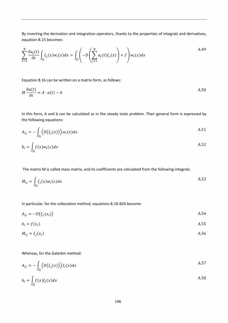
196
By inverting the derivation and integration operators, thanks to the properties of integrals and derivatives,
equation B.15 becomes:
A.49
Equation B.16 can be written on a matrix form, as follows:
A.50
In this form, A and b can be calculated as in the steady state problem. Their general form is expressed by
the following equations:
A.51
A.52
The matrix M is called mass matrix, and its coefficients are calculated from the following integrals:
A.53
In particular, for the collocation method, equations B.18-B20 become:
A.54
A.55
A.56
Whereas, for the Galerkin method:
A.57
A.58
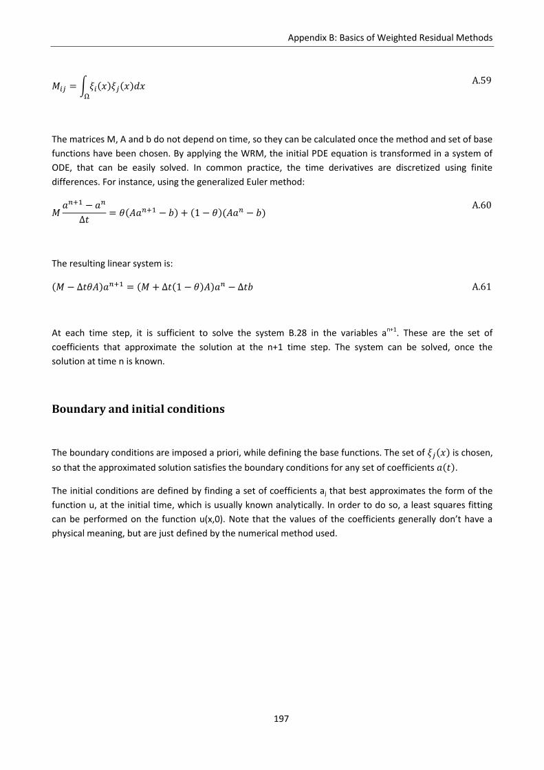
Appendix B: Basics of Weighted Residual Methods
197
A.59
The matrices M, A and b do not depend on time, so they can be calculated once the method and set of base
functions have been chosen. By applying the WRM, the initial PDE equation is transformed in a system of
ODE, that can be easily solved. In common practice, the time derivatives are discretized using finite
differences. For instance, using the generalized Euler method:
A.60
The resulting linear system is:
A.61
At each time step, it is sufficient to solve the system B.28 in the variables an+1. These are the set of
coefficients that approximate the solution at the n+1 time step. The system can be solved, once the
solution at time n is known.
Boundary and initial conditions
The boundary conditions are imposed a priori, while defining the base functions. The set of is chosen,
so that the approximated solution satisfies the boundary conditions for any set of coefficients .
The initial conditions are defined by finding a set of coefficients aj that best approximates the form of the
function u, at the initial time, which is usually known analytically. In order to do so, a least squares fitting
can be performed on the function u(x,0). Note that the values of the coefficients generally don’t have a
physical meaning, but are just defined by the numerical method used.

198
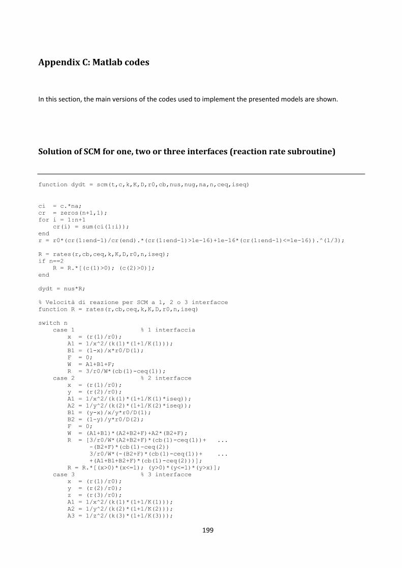
199
Appendix C: Matlab codes
In this section, the main versions of the codes used to implement the presented models are shown.
Solution of SCM for one, two or three interfaces (reaction rate subroutine)
function dydt = scm(t,c,k,K,D,r0,cb,nus,nug,na,n,ceq,iseq)
ci = c.*na;
cr = zeros(n+1,1);
for i = 1:n+1
cr(i) = sum(ci(1:i));
end
r = r0*(cr(1:end-1)/cr(end).*(cr(1:end-1)>1e-16)+1e-16*(cr(1:end-1)<=1e-16)).^(1/3);
R = rates(r,cb,ceq,k,K,D,r0,n,iseq);
if n==2
R = R.*[(c(1)>0); (c(2)>0)];
end
dydt = nus*R;
% Velocità di reazione per SCM a 1, 2 o 3 interfacce
function R = rates(r,cb,ceq,k,K,D,r0,n,iseq)
switch n
case 1 % 1 interfaccia
x = (r(1)/r0);
A1 = 1/x^2/(k(1)*(1+1/K(1)));
B1 = (1-x)/x*r0/D(1);
F = 0;
W = A1+B1+F;
R = 3/r0/W*(cb(1)-ceq(1));
case 2 % 2 interfacce
x = (r(1)/r0);
y = (r(2)/r0);
A1 = 1/x^2/(k(1)*(1+1/K(1)*iseq));
A2 = 1/y^2/(k(2)*(1+1/K(2)*iseq));
B1 = (y-x)/x/y*r0/D(1);
B2 = (1-y)/y*r0/D(2);
F = 0;
W = (A1+B1)*(A2+B2+F)+A2*(B2+F);
R = [3/r0/W*(A2+B2+F)*(cb(1)-ceq(1))+ ...
-(B2+F)*(cb(1)-ceq(2))
3/r0/W*(-(B2+F)*(cb(1)-ceq(1))+ ...
+(A1+B1+B2+F)*(cb(1)-ceq(2)))];
R = R.*[(x>0)*(x<=1); (y>0)*(y<=1)*(y>x)];
case 3 % 3 interfacce
x = (r(1)/r0);
y = (r(2)/r0);
z = (r(3)/r0);
A1 = 1/x^2/(k(1)*(1+1/K(1)));
A2 = 1/y^2/(k(2)*(1+1/K(2)));
A3 = 1/z^2/(k(3)*(1+1/K(3)));
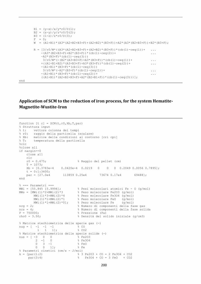
200
B1 = (y-x)/x/y*r0/D(1);
B2 = (z-y)/y/z*r0/D(2);
B3 = (1-z)/z*r0/D(3);
F = 0;
W = (A1+B1)*(A3*(A2+B2+B3+F)+(A2+B2)*(B3+F))+A2*(A3*(B2+B3+F))+B2*(B3+F);
R = [3/r0/W*((A3*(A2+B2+B3+F)+(A2+B2)*(B3+F))*(cb(1)-ceq(1))+ ...
-(A3*(B2+B3+F)+B2*(B3+F))*(cb(1)-ceq(2))+ ...
-A2*(B3+F)*(cb(1)-ceq(3)))
3/r0/W*(-(B2*(A3+B3+F)+A3*(B3+F))*(cb(1)-ceq(1))+ ...
+((A1+B1+B2)*(A3+B3+F)+A3*(B3+F))*(cb(1)-ceq(2))+ ...
-(A1+B1)*(B3+F)*(cb(1)-ceq(3)))
3/r0/W*(-A2*(B3+F)*(cb(1)-ceq(1))+ ...
-(A1+B1)*(B3+F)*(cb(1)-ceq(2))+ ...
((A1+B1)*(A2+B2+B3+F)+A2*(B2+B1+F))*(cb(1)-ceq(3)))];
end
Application of SCM to the reduction of iron process, for the system Hematite-
Magnetite-Wustite-Iron
function [t c] = SCM(t,r0,Xb,T,par)
% Struttura input
% t: vettore colonna dei tempi
% r0: raggio della particella (scalare)
% Xb: matrice delle condizioni al contorno [cri cpi]
% T: temperatura della particella
%clc
%close all
if nargin==0
close all
clc
r0 = 0.675; % Raggio del pellet (cm)
T = 1073;
Xb = [0.3783e-4 0.0420e-4 0.0219 0 0 0 0.2049 0.0056 0.7895];
t = 0:1:3600;
par = [27.0e4 113859 0.25e4 73674 0.17e4 69488];
end
% === Parametri ===
MWi = [55.845 15.9994]; % Pesi molecolari atomici Fe - O (g/mol)
MWs = [MWi(1)*2+MWi(2)*3 % Peso molecolare Fe2O3 (g/mol)
MWi(1)*3+MWi(2)*4 % Peso molecolare Fe3O4 (g/mol)
MWi(1)*1+MWi(2)*1 % Peso molecolare FeO (g/mol)
MWi(1)*1+MWi(2)*0]; % Peso molecolare Fe (g/mol)
ncg = 2; % Numero di componenti della fase gas
ncs = 4; % Numero di componenti della fase solida
P = 750000; % Pressione (Pa)
rho0 = 3.50; % Densità del solido iniziale (g/cm3)
% Matrice stechiometrica delle specie gas (-)
nug = [ -1 -1 -1 % CO
1 1 1]; % CO2
% Matrice stechiometrica delle specie solide (-)
nus = [ -3 0 0 % Fe2O3
2 -1 0 % Fe3O4
0 3 -1 % FeO
0 0 1]; % Fe
% Parametri cinetici (cm/s - J/mol)
k = [par(1:2) % 3 Fe2O3 + CO = 2 Fe3O4 + CO2
par(3:4) % Fe3O4 + CO = 3 FeO + CO2
Appendix C: Matlab codes
201
par(5:6) ]; % FeO + CO = Fe + CO2
% Parametri termodinamici (K)
K = [ 3.940 3968.37 % 3 Fe2O3 + CO = 2 Fe3O4 + CO2
8.980 -3585.64 % Fe3O4 + CO = 3 FeO + CO2
-2.946 2744.63]; % FeO + CO = Fe + CO2
% Matrice delle diffusività a 1 atm, 1073 K (cm2/s)
D = [1.0 1.5 1.8 % CO-CO CO-CO2 CO-N2
1.5 1.0 1.5 % CO2-CO CO2-CO2 CO2-N2
1.8 1.5 1.0]; % N2-CO N2-CO2 N2-N2
h = 30.0; % Coefficiente scambio materia (cm/s)% Conducibilità dei
gas (W/mK)
por0 = [0.3396; 0.3431; 0.4475; 0.6890];
kd = k(:,1).*exp(-k(:,2)/T/8.314);
cd = 101325./P.*(T./1073).^1.75.*(1/2.*por0.*(1+por0));
Dif = D(1,2).*cd;
Keq = exp(K(:,1)+K(:,2)./T);
cg0 = Xb(1:2);
cs0 = Xb(3:6);
xb = Xb(7:end);
Di = (1-xb)./(xb*(1./D)-xb./diag(D,0)');
cFeMax = sum(cs0.*[2 3 1 1]);
[t c] = ode45(@scm,t,cs0,[],kd,Keq,Dif,cFeMax,r0,cg0,nus);
%plot(t,c)
cH = c(:,1);
cM = c(:,2);
cW = c(:,3);
cF = c(:,4);
r3 = r0*(1-cF./cFeMax).^(1/3);
r2 = r0*((2*cH+3*cM)./cFeMax).^(1/3);
r1 = r0*(2*cH./cFeMax).^(1/3);
x = r1/r0;
y = r2/r0;
z = r3/r0;
plot(t,x,t,y,t,z),legend('r_1/r_0','r_2/r_0','r_3/r_0'),xlabel('t')
figure
plot(t,cH,t,cM,t,cW,t,cF),legend('Fe_2O_3','Fe_3O_4','FeO','Fe'),xlabel('t')
xlim([0 t(end)]),ylim([0 0.04])
function dcdt = scm(t,c,kd,Keq,Dif,cFeMax,r0,cgb,nus)
cH = c(1);
cM = c(2);
cW = c(3);
cF = c(4);
r3 = r0*((1-cF/cFeMax)*(cF<cFeMax)+1e-16*(cF>=cFeMax))^(1/3);
r2 = r0*((2*cH+3*cM)/cFeMax*(2*cH+3*cM>0)+1e-16*(2*cH+3*cM<0))^(1/3);
r1 = r0*(2*cH/cFeMax*(cH>0)+1e-16*(cH<=0))^(1/3);
x = (r1/r0);
y = (r2/r0);
z = (r3/r0);
A1 = 1/x^2/(kd(1)*(1+1/Keq(1)));
A2 = 1/y^2/(kd(2)*(1+1/Keq(2)));
A3 = 1/z^2/(kd(3)*(1+1/Keq(3)));
B1 = (y-x)/x/y*r0/Dif(2);
B2 = (z-y)/y/z*r0/Dif(3);
B3 = (1-z)/z*r0/Dif(4);
F = 0;
W = (A1+B1)*(A3*(A2+B2+B3+F)+(A2+B2)*(B3+F))+A2*(A3*(B2+B3+F))+B2*(B3+F);
ceq1 = (cgb(1)+cgb(2))/(1+Keq(1));
ceq2 = (cgb(1)+cgb(2))/(1+Keq(2));
ceq3 = (cgb(1)+cgb(2))/(1+Keq(3));
R1 = 3/r0/W*((A3*(A2+B2+B3+F)+(A2+B2)*(B3+F))*(cgb(1)-ceq1)+...
202
-(A3*(B2+B3+F)+B2*(B3+F))*(cgb(1)-ceq2)+...
-A2*(B3+F)*(cgb(1)-ceq3));
R2 = 3/r0/W*(-(B2*(A3+B3+F)+A3*(B3+F))*(cgb(1)-ceq1)+...
+((A1+B1+B2)*(A3+B3+F)+A3*(B3+F))*(cgb(1)-ceq2)+...
-(A1+B1)*(B3+F)*(cgb(1)-ceq3));
R3 = 3/r0/W*(-A2*(B3+F)*(cgb(1)-ceq1)+...
-(A1+B1)*(B3+F)*(cgb(1)-ceq2)+...
((A1+B1)*(A2+B2+B3+F)+A2*(B2+B1+F))*(cgb(1)-ceq3));
dcdt = (nus*[R1*(R1>0); R2*(R2>0); R3*(R3>0)]);
Application of the continuous model applied to the process reduction of iron.
Single particle model, coupled with moving bed reactor model.
function PelletFullPFRDiff
clc
close all
global p
global m
global bc
global ic
global solve
% === Parametri ===
p.MWs = [159.6882; 231.5326; 71.8444; 55.8450]; % Pesi
molecolari dei solidi (g/mol)
p.MWg = [28.01010; 44.00950; 28.01340]; % Pesi
molecolari dei gas (g/mol)
p.r0 = 0.675; % Raggio del
pellet (cm)
p.ncg = 2; % Numero di
reagenti della fase gas
p.ncs = 4; % Numero di
componenti della fase solida
% p.rho0 = 3.50; % Densità
del solido iniziale (g/cm3)
p.rho0 = 5.29; % Densità del
solido iniziale (g/cm3)
p.rhoi = [5.30; 5.15; 5.70; 7.87]; % Densità
intrinseche dei solidi (g/cm3)
p.a0 = [10.0; 2.96; 0.65; 0.40]*10^4*p.rho0; % Rapporto
superficie/volume per i solidi puri (1/cm)
p.ps = [1.72 1.56 2.00 1.50]; % Costanti di
sinterizzazione
p.kg = [0.0240; 0.0146; 0.0240]; %
Conducibilità dei gas (W/mK)
p.ks = [80.2; 80.2; 80.2; 80.2]; %
Conducibilità dei solidi (W/mK)
p.Cpg = [1.185; 1.234; 1.185]; % Calori
specifici dei gas (J/gK)
p.Cps = [1.07; 1.07; 0.82; 0.83]; % Calori
specifici dei solidi (J/gK)
p.h = 30.0; %
Coefficiente scambio materia (cm/s)
p.ht = 0.20*4.18; %
Coefficiente di scambio termico alla parete (W/cm2K)
p.L = 10; % Altezza del
reattore (m)
p.d = 1; % Diametro
del reattore (m)
p.us = 0.002; % Velocità
di discesa del solido (m/s)
Appendix C: Matlab codes
203
p.m0 = 2; % Portata
massiva di gas alimentato (kg/s)
p.porx = 0.47; % Porosità
del letto
p.Np = (1-p.porx)/(4/3*pi*(p.r0*1e-2)^3); % Numero di
pellet per unità di volume (1/m3tot)
p.rhod = 4.23;
p.MWd = 79.866;
p.yd = 0.46;
% Matrice stechiometrica delle specie gas (-)
p.nug = [ -1 -1 -1 % CO
1 1 1]; % CO2
% Matrice stechiometrica delle specie solide (-)
p.nus = [ -3 0 0 % Fe2O3
2 -1 0 % Fe3O4
0 3 -1 % FeO
0 0 1]; % Fe
% Parametri cinetici (cm/s - J/mol)
p.k = [221.82e-4 5514.7*8.314 % 3 Fe2O3 + CO = 2 Fe3O4 + CO2
704.03e-4 6098.6*8.314 % Fe3O4 + CO = 3 FeO + CO2
916.20e-4 2036.5*8.314];% FeO + CO = Fe + CO2
% Parametri termodinamici (K)
p.K = [3.940 3968.37 % 3 Fe2O3 + CO = 2 Fe3O4 + CO2
8.980 -3585.64 % Fe3O4 + CO = 3 FeO + CO2
-2.946 2744.63]; % FeO + CO = Fe + CO2
% Matrice delle diffusività a 1 atm, 1073 K (cm2/s)
p.D = [1.0 1.5 1.8 % CO-CO CO-CO2 CO-N2
1.5 1.0 1.5 % CO2-CO CO2-CO2 CO2-N2
1.8 1.5 1.0]; % N2-CO N2-CO2 N2-N2
% Parametri per la viscosità
p.mu0 = [118 518.67 0.01720 % CO
240 527.67 0.01480 % CO2
111 540.99 0.01781]; % N2
% Parametri per i calori di reazione dH = a + b*(T-c)
p.dH = [-3000 -3.18 1023 % 3 Fe2O3 + CO = 2 Fe3O4 + CO2
13500 0 0 % Fe3O4 + CO = 3 FeO + CO2
-3975 -0.90 673]; % FeO + CO = Fe + CO2
% === Creazione mesh ===
m.ns = 100; % Numero di
celle
m.nt = 100; % Numero di
tempi
m.rb = linspace(0,p.r0,m.ns+1)'; % Coordinate
dei bordi delle celle nel pellet (cm)
m.r = (m.rb(2:end)+m.rb(1:end-1))/2; % Coordinate
dei nodi nel pellet (cm)
m.z = linspace(0,p.L,m.nt); %
Discretizzazione spaziale del reattore (m)
m.t = m.z/p.us; %
Discretizzazione del tempo (s)
% === Condizioni al contorno ===
bc.Tb = 1073; % Temperatura
di bulk (K)
bc.Pb = 750000; % Pressione
di bulk (Pa)
bc.cb = bc.Pb/8.314/bc.Tb*10^-6; %
Concentrazione totale di bulk (mol/cm3)
bc.xend = [0.4 0.0 0.6];
bc.cgb = bc.xend(1:end-1)*bc.cb; %
Concentrazioni dei gas di bulk (mol/cm3)
bc.cs0 = [p.rho0/p.MWs(1) 0 0 0]; %
Concenrazioni dei solidi (mol/cm3)
bc.rhouend = -p.m0/(p.d^2/4*pi); %kg/m2tot/s
% === Condizioni iniziali ===
204
ic.cg0 = repmat([0.0 0.0],m.ns,1)*bc.cb; %
Composizione fase gas nel pellet (mol/cm3)
ic.cs0 = repmat(bc.cs0,m.ns,1); %
Composizione fase solida nel pellet (mol/cm3)
ic.T0 = ones(m.ns,1)*bc.Tb; % Temperature
iniziali (K)
ic.por0 = epps(ic.cs0,[],p.MWs,p.rhoi,m.ns,p.ncs); % Porosità
iniziale
ic.cgpor0 = ic.cg0.*repmat(ic.por0,1,p.ncg); % Prodotto
concentrazioni-porosità iniziale
% === Setting modello ===
solve.pfr = false;
% Modello di diffusione
% F: Fick, diffusività binaria
% MA: Fick, diffusività Mixture-Averaged
% SM: Stefan-Maxwell
modelD = 'SM';
% Modello termico
% ISOT: Isotermo, temperatura omogenea, uguale a quella di bulk
% ADIAB: Adiabatico, scambio termico nullo alla parete
% BT: Temperatura fissa alla parete, uguale a quella di bulk
% FLUX: Flusso termico alla parere, secondo la legge q = ht*(Tb-T)
modelT = 'FLUX';
% Esecuzione del calcolo
% true: Esegue l'integrazione temporale e post processing
% false: Carica i risultati ed esegue post processing e bilanci di materia
docalc = true;
doplot = true;
% === Inizializzazioni ===
m.Afv = 3*[-m.rb(1:end-1)./(m.rb(2:end).^3-m.rb(1:end-1).^3)... % Diagonale -
1 della matrice dei volumi finiti
m.rb(2:end)./(m.rb(2:end).^3-m.rb(1:end-1).^3)]; % Diagonale
0 della matrice dei volumi finiti
m.Afv = spdiags(m.Afv,[1 0],m.ns,m.ns)'; % Matrice
sparsa dei volumi finiti per divergenza in geometria sferica
X0 = [reshape(ic.cgpor0,[],1) % Condizioni
iniziali per il bilancio fase gas
reshape(ic.cs0,[],1) % Condizioni
iniziali per il bilancio fase solida
reshape(ic.T0,[],1)]; % Condizioni
iniziali per il bilancio termico
Xend = [bc.rhouend % Condizioni
finali per l'equazione di continuità di bulk
bc.xend(1:end-1)']; % Condizioni
finali per il bilancio in fase gas di bulk
% === Calcolo ===
if docalc==true
if solve.pfr
omega = 0.05; % Fattore di
rilassamento
nmax = 100; % Numero
massimo di iterazioni
toll = 1e-4; % Tolleranza
x = Xend; % Inizializza
le condizioni iniziali non note
%x = [-15.510; 0.0176; 0.3822];
err = 1; % Inizializza
l'errore
n = 1; % Inizializza
il numero di iterazioni
tic
while err>toll && n<nmax
Appendix C: Matlab codes
205
fprintf('\n N. iterazione: %3.0f \n',n)
R = res(x,m.t,X0,Xend,modelD,modelT); % Risolve ai
valori iniziali e calcola il residuo
err = norm(R); % Funzione
errore
x = x+omega*R; % Valore
delle incognite alla nuova iterazione
n = n+1; %
Aggiornamento del contatore
end
x = [x; 1-sum(x(end-p.ncg+1:end)); zeros(p.ncg+1,1)]; %
Composizione della soluzione
[~, X] = ode15s(@DAEfun,m.t,[X0; x],[],modelD,modelT,false); % Risoluzione
dei bilanci con i valori al contorno corretti
etime = toc; % Tempo di
calcolo (s)
fprintf('\n Tempo di calcolo: %3.2f s\n',etime)
else
x = Xend;
x = [x; 1-sum(x(end-p.ncg+1:end)); zeros(p.ncg+1,1)]; %
Composizione della soluzione
[~, X] = ode15s(@DAEfun,m.t,[X0; x],[],modelD,modelT,false);
end
save('pelletPFRDiffArt.mat','X','X0','x','p','m','bc') % Salva le
soluzioni
else
load 'pelletPFRDiffArt.mat' % Carica
le soluzioni
end
% === Post Processing ===
rhou = -flipud(X(:,m.ns*(p.ncg+p.ncs+1)+1));
xbulk = flipud(X(:,m.ns*(p.ncg+p.ncs+1)+2:m.ns*(p.ncg+p.ncs+1)+2+p.ncg));
j = flipud(X(:,m.ns*(p.ncg+p.ncs+1)+1+(p.ncg+1)+1:end));
rho = xbulk*p.MWg*bc.cb*1e3;
u = rhou./rho;
cs = X(:,m.ns*p.ncg+1:m.ns*(p.ncg+p.ncs));
%n(m.t(1),X(1,:)',modelD,modelT,doplot)
subplot(3,2,[2 4 6])
plot(xbulk,m.z),xlabel('x_i'),ylabel('z (m)'),legend('CO','CO_2','N_2'),xlim([0 0.7])
csI = reshape(cs(round(1/100*m.nt),:),m.ns,p.ncs);
subplot(3,2,1)
plot(m.r/m.r(end),csI),ylabel(sprintf('z = %3.1f m',m.z(round(99/100*m.nt))))
legend('Fe_2O_3','Fe_3O_4','FeO','Fe','Location','NorthWest')
csI = reshape(cs(round(1/2*m.nt),:),m.ns,p.ncs);
subplot(3,2,3)
plot(m.r/m.r(end),csI),ylabel(sprintf('z = %3.1f m',m.z(round(1/2*m.nt))))
csI = reshape(cs(round(1/1*m.nt),:),m.ns,p.ncs);
subplot(3,2,5)
plot(m.r/m.r(end),csI),ylabel(sprintf('z = %3.1f m',m.z(1))),xlabel('r/R')
figure
plot(m.z,j)
figure
plot(m.z,u)
m.t
% cs0 = reshape(cs(1,:),[],4);
% m0 = trapz(m.r,4*pi*m.r.^2.*(cs0*p.MWs));
% mend = trapz(m.r,4*pi*m.r.^2.*(csI*p.MWs));
% % u(end)*(D^2/4*pi)*cbulk(end)*1e6*xbulk(1,2).*16*1e-3
% mpin = p.us*(p.d^2/4*pi).*p.Np*m0*1e-3
% mpout = p.us*(p.d^2/4*pi).*p.Np*mend*1e-3
% mpin-mpout
%
% mgin = rhou(1)*pi*p.d^2/4
% mgout = rhou(end)*pi*p.d^2/4
206
% mgout-mgin
% figure
% plot(m.z,j)
% =========================================================================
% Costruzione dei bilanci di materia ed energia
% =========================================================================
function B = DAEfun(t,X,modelD,modelT,doplot)
global p
global m
global bc
global solve
% Estrazione delle variabili dipendenti
cgpor = reshape(X(1:m.ns*p.ncg),m.ns,p.ncg); % Matrice
delle concentrazioni in fase gas (mol/cm3tot)
cs = reshape(X(m.ns*p.ncg+1:m.ns*(p.ncg+p.ncs)),m.ns,p.ncs); % Matrice
delle concentrazioni in fase solida (mol/cm3tot)
T = X(m.ns*(p.ncg+p.ncs)+1:m.ns*(p.ncg+p.ncs+1)); % Vettore
delle temperature (K)
rhou = X(m.ns*(p.ncg+p.ncs+1)+1); % Flusso
massivo di bulk (kg/m2tot/s)
xbulk = X(m.ns*(p.ncg+p.ncs+1)+2:m.ns*(p.ncg+p.ncs+1)+2+p.ncg)'; % Frazioni
massive dei gas di bulk
jbulk = X(m.ns*(p.ncg+p.ncs+1)+1+(p.ncg+1)+1:end); % Flussi
diffusivi massivi dei gas di bulk (kg/m2tot/s)
xbulk = xbulk.*(xbulk>0)+ones(1,p.ncg+1)*1e-10.*(xbulk<=0); % Porta a
zero le frazioni negative
xbulk = xbulk/sum(xbulk); %
Rinormalizza sulla somma a 1
ybulk = xbulk.*p.MWg'/(xbulk*p.MWg); % Frazioni
massive dei gas di bulk
% Variabili ai nodi
[por rho] = epps(cs,[],p.MWs,p.rhoi,m.ns,p.ncs); % Campo di
porosità (-) e densità apparente (g/cm3)
c = bc.Pb/8.314./T*10^-6; % Matrice
della concentrazione totale di gas (mol/cm3gas)
cg = cgpor./repmat(por,1,p.ncg); % Matrice
delle concentrazioni in fase gas (mol/cm3gas)
xg = [cg./repmat(c,1,p.ncg) 1-sum(cg./repmat(c,1,p.ncg),2)]; % Frazioni
molari dei gas
xs = cs./repmat(sum(cs,2),1,p.ncs); % Frazioni
molari dei solidi
P = c*1e6*8.314.*T; % Campo di
pressione (Pa)
ktg = xg*p.kg/100; %
Conducibilità della fase gas (W/cm/K)
kts = xs*p.ks/100; %
Conducibilità della fase solida (W/cm/K)
kt = ktg.*por+kts.*(1-por); %
Conducibilità del medium (W/cm/K)
Cpg = xg*p.Cpg; % Cp della
fase gas (J/gK)
Cps = xs*p.Cps; % Cp della
fase solida (J/gK)
Cp = Cpg.*por+Cps.*(1-por); % Cp del
medium (J/gK)
DH = (repmat(p.dH(:,1)',m.ns,1)+repmat(p.dH(:,2)',m.ns,1).*... % Calori di
reazione (J/mol)
(repmat(T,1,size(p.dH,1))-repmat(p.dH(:,3)',m.ns,1)))*4.18;
% Estrapolazioni al contorno
nfit = 3; % Grado del
polinomio da utilizzare
Appendix C: Matlab codes
207
pb = polyval(polyfit(m.r(end-nfit:end),por(end-nfit:end),nfit),m.rb(end)); % Porosità a
r = R (-)
kb = polyval(polyfit(m.r(end-nfit:end),kt(end-nfit:end),nfit),m.rb(end)); %
Conducibilità a r = R (W/cm/K)
% Variabili ai bordi delle celle
porb = [por(1); Davg(por(1:end-1),por(2:end)); pb]; % Porosità
ktb = [kt(1); Davg(kt(1:end-1),kt(2:end)); kb]; %
Conducibilità (W/cm/K)
[T0 x0] = BC(bc.Tb,bc.Pb,xbulk,m.rb(end)-m.r(end),p.ncg,... % Temperatura
e composizione alla parete
modelT,modelD,T(end),xg(end,:),ktb(end),porb(end),p.D,p.ht,p.h);
xgb = [xg(1,:); Davg(xg(1:end-1,:),xg(2:end,:)); x0]; % Frazioni
molari dei gas
xgb = xgb./repmat(sum(xgb,2),1,p.ncg+1); % Normalizza
le frazioni molari interpolate
MWgb = xgb*p.MWg; % Peso
molecolare della fase gas (g/mol)
ygb = xgb.*repmat(p.MWg',m.ns+1,1)./repmat(MWgb,1,p.ncg+1); % Frazioni
massive dei gas
Tb = [T(1); Davg(T(1:end-1),T(2:end)); T0]; % Temperature
(K)
Pb = [P(1); Davg(P(1:end-1),P(2:end)); bc.Pb]; % Pressione
(Pa)
cb = [c(1); Davg(c(1:end-1),c(2:end)); bc.Pb/8.314/T0*10^-6]; %
Concentrazione totale di gas (mol/cm3gas)
cD = 101325./Pb.*(Tb./1073).^1.75.*(1/2.*porb.*(1+porb)); % Correzione
diffusività in base a T, P, porosità
% Gradienti ai bordi delle celle
gradT = [0; % Gradiente
di temperatura a r = 0
(T(2:end)-T(1:end-1))./(m.r(2:end)-m.r(1:end-1)); % Gradiente
di temperatura a 0<r<R
(Tb(end)-T(end))/(m.rb(end)-m.r(end))]; % Gradiente
di temperatura a r = R
gradx = [zeros(1,p.ncg+1); % Gradiente
delle x a r = 0
(xg(2:end,:)-xg(1:end-1,:))./repmat(m.r(2:end)-m.r(1:end-1),1,p.ncg+1); %
Gradiente delle x a 0<r<R
(xgb(end,:)-xg(end,:))./(m.rb(end)-m.r(end))]; % Gradiente
delle x a r = R
% Termini di generazione
R = Rrate(p.k,p.K,cg,cs,T,m.ns,p.a0,p.ps); % Velocità di
reazione (mol/cm3/s)
rpg = (p.nug*R')'; % Velocità di
produzione dei gas (mol/cm3/s)
rps = (p.nus*R')'; % Velocità di
produzione dei solidi (mol/cm3/s)
Q = -sum(DH.*R,2); % Produzione
di calore (W/cm3)
% Bilancio termico
q = thfluxes(gradT,ktb); % Flusso
conduttivo (W/cm2)
divq = divf(q,m.rb,1); % Divergenza
del flusso conduttivo (W/cm3)
dTdt = (-divq+Q)./(rho.*Cp)*(strcmp(modelT,'ISOT')==0); % Derivata
della temperatura (K/s)
% Bilancio di concentrazione totale
[~, ~, dpordt] = epps(cs,rps,p.MWs,p.rhoi,m.ns,p.ncs); % Derivata
della porosità (1/s)
dPdt = zeros(m.ns,1); % Derivata
della pressione (Pa/s)
dcdt = 1/8.314./T.^2.*(T.*dPdt-P.*dTdt)*1e-6; % Derivata
della concentrazione totale di gas (mol/cm3gas/s)
208
dcpordt = dpordt.*c+por.*dcdt; % Derivata
della concentrazione totale di gas (mol/cm3tot/s)
Nt = [0; m.Afv\(-dcpordt+sum(rpg,2))]; % Flusso
molare totale di gas (mol/cm2/s)
% Bilanci di specie chimica
J = fluxes(modelD,xgb,gradx(:,1:end-1),repmat(cb,1,p.ncg),p.D,cD,m.ns+1,p.ncg+1); %
Flussi diffusivi molari di gas (mol/cm2/s)
N = repmat(Nt,1,p.ncg+1).*xgb+J; % Flussi
molari totali delle singole specie gas (mol/cm2/s)
divN = divf(N(:,1:end-1),m.rb,p.ncg); % Divergenza
dei flussi molari delle specie gas (mol/cm3/s)
dcgdt = -divN+rpg; % Derivate
delle concentrazioni delle specie gas (mol/cm3/s)
dcsdt = rps; % Derivate
delle concentrazioni delle specie solide (mol/cm3/s)
% Campi di velocità nel pellet
vstar = Nt./cb; % Velocità
molare del gas (cm/s)
v = vstar+sum(ygb./xgb.*J./repmat(cb,1,p.ncg+1),2); % Velocità
del gas (cm/s)
if solve.pfr
% Bilanci di bulk
rbulk = N(end,:)'.*p.MWg*4*pi*m.rb(end)^2*1e-3*p.Np; % Produzione
massiva delle specie gas di bulk (kg/m3tot/s)
MWbulk = xbulk*p.MWg; % Peso
molecolare del gas di bulk (kg/kmol)
rhobulk = cb(end)*MWbulk*1e3; % Densità del
gas di bulk (kg/m3)
Db = p.D*1e-4*101325/bc.Pb*(bc.Tb/1073)^1.75; % Matrice
delle diffusività di bulk (m2/s)
Bj = SM('j',Db,p.ncg+1,xbulk,ybulk); % Matrice S-M
per i flussi massivi (s/m2)
dxdz = -1/rhobulk*Bj*jbulk(1:end-1); % Gradienti
di x bulk (1/m)
dxdz = [dxdz; -sum(dxdz)]; % Completa la
matrice dei gradienti di x bulk
Bxy = xy('xy',p.ncg+1,p.MWg,MWbulk,xbulk,ybulk); % Matrice di
conversione da gradienti molari a massivi
dydz = [Bxy*dxdz(1:end-1); -sum(Bxy*dxdz(1:end-1))]; % Gradienti
di y bulk (1/m)
drhoudt = p.us*sum(rbulk); % Derivata
temporale del flusso massivo totale (kg/m2tot/s2)
dxdt = p.us*dxdz; % Derivate
temporali di x bulk (1/s)
djdt = p.us*(rbulk-rhou*dydz-ybulk'*sum(rbulk)); % Derivate
temporali dei flussi diffusivi massivi (kg/m2tot/s2)
djdt(end) = -sum(djdt(1:end-1)); % Impone
nulla la somma delle derivate dei flussi siffusivi
% Composizione dei bilanci
B = [reshape(dcgdt,[],1); % Bilanci di
concentrazione in fase gas (mol/cm3/s)
reshape(dcsdt,[],1); % Bilanci di
concentrazione in fase solida (mol/cm3/s)
dTdt % Bilancio
termico (K/s)
drhoudt % Equazione
di continuità di bulk (kg/m2tot/s2)
dxdt % Bilancio
delle frazioni massive di bulk (1/s)
djdt]; % Bilancio
dei flussi diffusivi massivi di bulk (kg/m2tot/s2)
else
B = [reshape(dcgdt,[],1); % Bilanci di
concentrazione in fase gas (mol/cm3/s)
Appendix C: Matlab codes
209
reshape(dcsdt,[],1); % Bilanci di
concentrazione in fase solida (mol/cm3/s)
dTdt; % Bilancio
termico (K/s)
zeros(2*length(xbulk)+1,1)];
end
% Progresso del calcolo
H = waitbar(t/m.t(end)); % Crea la
barra
waitbar(t/m.t(end),H,sprintf('%2.1f %%',t/m.t(end)*100)); % Segnala il
progresso
if t == m.t(end)
close(H) % Chiude la
barra alla fine
end
% Plotting dei profili
if doplot
subplot(241)
plot(m.rb/m.rb(end),xgb)
ylabel('X gas'),legend('CO','CO_2','N_2')
subplot(242)
plot(m.r/m.rb(end),cs)
ylabel('c solidi (mol/cm3)'),legend('Hem','Mag','Wus','Fe')
subplot(243)
plot(m.rb/m.rb(end),Tb)
ylabel('T (K)')
subplot(244)
plot(m.rb/m.rb(end),Nt)
ylabel('Flusso molare totale (mol/cm2/s)')
subplot(245)
plot(m.rb/m.rb(end),porb)
ylabel('porosità')
subplot(246)
plot(m.rb/m.rb(end),cb)
ylabel('c totale gas (mol/cm3)')
subplot(247)
plot(m.rb/m.rb(end),J(:,1),m.rb/m.rb(end),N(:,1),m.rb/m.rb(end),Nt)
ylabel('Flussi molari CO (mol/cm2/s)'),legend('J*','N','N_t')
subplot(248)
plot(m.rb/m.rb(end),v,m.rb/m.rb(end),vstar)
ylabel('velocità del gas (cm/s)'),legend('v','v*')
drawnow
end
%plot(m.rb,xgb,m.rb(end),xbulk,'o'),title(sprintf('progress = %3.2g
%%',t/m.t(end)*100)),drawnow
% =========================================================================
% Calcolo delle variabili al contorno
% =========================================================================
function [T0 x0] = BC(Tbulk,Pbulk,xbulk,dr,ncg,modelT,modelD,Tend,xend,k,por,D,ht,h)
T0 = Tbulk*(strcmp(modelT,'TB')+strcmp(modelT,'ISOT'))+ ... % Temperatura
di parete: Caso temperatura fissa alla parete
(Tend+Tbulk*dr*ht/k)/(1+dr*ht/k)*strcmp(modelT,'FLUX')+ ... % Temperatura
di parete: Caso flusso termico alla parete
Tend*strcmp(modelT,'ADIAB'); % Temperatura
di parete: Caso senza scambio termico alla parete
c0 = Pbulk/8.314/T0*10^-6; %
Concentrazione totale di gas alla parete (mol/cm3gas)
cD = 101325/Pbulk*(T0/1073)^1.75*(1/2*por*(1+por)); % Correzione
diffusività in base a T, P, porosità alla parete
x0 = xbulk; %
Composizione alla parete di primo tentativo
err = 1; % Inizializza
il calcolo iterativo della composizione alla parete
210
while err>1e-5
gradx0 = (x0(1:end-1)-xend(1:end-1))/dr; % Gradiente
di composizione alla parete
Jb = fluxes(modelD,x0,gradx0,repmat(c0,1,ncg),D,cD,1,ncg+1); % Flussi
diffusivi alla parete
x0new = xbulk+Jb./h./c0; %
Composizione alla parete uguagliando i flussi diffusivi ai flussi esterni
err = norm((x0new-x0)./x0); % Calcolo
dell'errore
x0 = (x0new+x0)/2; %
Aggiornamento delle composizioni alla parete
end
% =========================================================================
% Calcolo del campo di porosità
% =========================================================================
function [por rhoa dpordt] = epps(c,dcdt,MW,rhoi,ns,nc)
rhoa = c*MW; % Densità
apparente (g/cm3)
y = c.*repmat(MW',ns,1)./repmat(rhoa,1,nc); % Frazioni
massive di solido
rhot = 1./(y*(1./rhoi)); % Densità
teorica (g/cm3)
por = 1-rhoa./rhot; % Campo di
porosità
if nargout==3
sdcMWdt = dcdt*MW; % Derivata
della densità apparente (g/cm3/s)
dydt = zeros(ns,nc); % Inizializza
le derivate delle frazioni massive
for i=1:nc
dydt(:,i)=(dcdt(:,i).*MW(i).*rhoa-c(:,i).*MW(i).*sdcMWdt)./rhoa.^2; % Derivate
delle frazioni massive (1/s)
end
drhotdt = -(dydt*(1./rhoi)).*rhot.^2; % Derivata
della densità teorica (g/cm3/s)
drhoadt = sdcMWdt; % Derivata
della densità apparente (g/cm3/s)
dpordt = -(drhoadt.*rhot-rhoa.*drhotdt)./rhot.^2; % Derivata
della porosità (1/s)
end
% =========================================================================
% Calcolo delle velocità di reazione --> Meccanismo cinetico
% =========================================================================
function R = Rrate(k,K,cg,cs,T,ns,a0,p)
xs = repmat([2 3 1 1],ns,1).*cs./repmat(cs*[2 3 1 1]',1,4); % Conversioni
locali delle specie solide (-)
a = repmat(a0',ns,1).*xs.^repmat(p,ns,1); % Aree
superficiali per le fasi solide (1/cm)
kr = repmat(k(:,1)',ns,1).*exp(-repmat(k(:,2)',ns,1)/8.314./repmat(T,1,3)); % Costanti
cinetiche (cm/s)
% Velocità di reazione (mol/cm3/s)
R(:,1) = kr(:,1).*(a(:,1).*cg(:,1)-a(:,2).*cg(:,2)./exp(K(1,1)+K(1,2)./T)); % Hematite -
-> Magnetite
R(:,2) = kr(:,2).*(a(:,2).*cg(:,1)-a(:,3).*cg(:,2)./exp(K(2,1)+K(2,2)./T)); % Magnetite -
-> Wustite
R(:,3) = kr(:,3).*(a(:,3).*cg(:,1)-a(:,4).*cg(:,2)./exp(K(3,1)+K(3,2)./T)); % Wustite -
-> Ferro
R = real(R); % Pulisce
eventuali parti immaginarie
% =========================================================================
% Calcolo dei flussi diffusivi
Appendix C: Matlab codes
211
% =========================================================================
function J = fluxes(model,x,gradx,c,D,cD,ns,n)
J = zeros(ns,n); % Inizializza
i flussi
switch model
% Diffusione Fickiana, binaria
case 'F'
Df = D(1,2)*repmat(cD,1,n-1); % Correzione
P, T, por
J(:,1:end-1) = -c.*Df.*gradx; % Legge di
Fick
% Diffusione Fickiana, diffusività Mixture-Averaged
case 'MA'
D0 = (1-x)./(x*(1./D)-x./repmat(diag(D,0)',ns,1)); % Regola di
miscela
Dma = D0(:,1:end-1).*repmat(cD,1,n-1); % Correzione
P, T, por
J(:,1:end-1) = -c.*Dma.*gradx; % Legge di
Fick
% Diffusione Stefan-Maxwell
case 'SM'
for k=1:ns
Dk = D*cD(k); % Correzione
P, T, por
xk = x(k,:); % Estrae la
composizione al raggio rk
Bk = SM('J',Dk,n,xk); % Calcolo
della matrice B
Dsm = Bk^-1; % Inversione
della matrice B
J(k,1:end-1) = -(c(k,:)'.*(Dsm*gradx(k,:)'))'; % Legge di
Fick generalizzata
end
end
J(:,end) = -sum(J(:,1:end-1),2); % Calcola i
flussi dell'ultima specie per differenza a zero
% =========================================================================
% Matrici di diffusività Stefan-Maxwell
% =========================================================================
function B = SM(flux,D,n,x,y)
B = zeros(n-1,n-1); % Inizializza
switch flux
case 'J' % Matrice per
i flussi molari
for i=1:n-1
for j=1:n-1
B(i,j) = x(i)/D(i,n)+ ... % Termini
comuni
(sum(x./D(i,:))-x(i)/D(i,i))*(i==j)+ ... % Termini
della diagonale
-x(i)/D(i,j)*(i~=j); % Termini
fuori dalla diagonale
end
end
case 'j' % Matrice per
i flussi massivi
for i=1:n-1
for j=1:n-1
B(i,j) = x(i)/y(j)*(y(j)/D(i,n)*x(n)/y(n)+ ... % Termini
comuni
(sum(x./D(i,:))-x(i)/D(i,i))*(i==j)+ ... % Termini
della diagonale
-x(j)/D(i,j)*(i~=j)); % Termini
fuori dalla diagonale
end
212
end
end
% =========================================================================
% Matrici di conversione dei gradienti di frazioni
% =========================================================================
function Bxy = xy(dir,n,MWi,MW,x,y)
Bxy = zeros(n-1,n-1); % Inizializza
switch dir
case 'xy'
for i=1:n-1
for j=1:n-1
Bxy(i,j) = MWi(i)/MW*((i==j)+x(i)/MW*(MWi(n)-MWi(j))); % Matrice per
passare dai gradienti di x ai gradienti di y
end
end
case 'yx'
for i=1:n-1
for j=1:n-1
Bxy(i,j) = MW/MWi(i)*((1==j)+y(i)*MW*(1/MWi(n)-1/MWi(j))); % Matrice per
passare dai gradienti di y ai gradienti di x
end
end
end
% =========================================================================
% Calcolo dei flussi conduttivi
% =========================================================================
function q = thfluxes(gradT,k)
q = -k.*gradT; % Legge di
Fourier
% =========================================================================
% Calcolo delle divergenze dei flussi
% =========================================================================
function df = divf(f,r,nb)
% Estensione della matrice dei raggi in base al numero di bilanci
r = repmat(r,1,nb); % Matrice
delle coordinate dei bordi (cm)
% Applicazione dei volumi finiti
df = 3*(r(2:end,:).^2.*f(2:end,:)-r(1:end-1,:).^2.*f(1:end-1,:))./ ... % Differenza
dei flussi
(r(2:end,:).^3-r(1:end-1,:).^3); % Divide per
il volume
% =========================================================================
% Calcolo delle variabili ai bordi
% =========================================================================
function D = Davg(D1,D2)
model = 'armonica'; % Modello
utilizzato
switch model
case 'aritmetica'
D = (D1+D2)./2; % Media
aritmetica
case 'armonica'
D = 2./(1./D1+1./D2); % Media
armonica
end
% =========================================================================
% Calcolo dei residui
% =========================================================================
function res = bcfun(ya,yb,modelD,modelT,doplot)
global bc
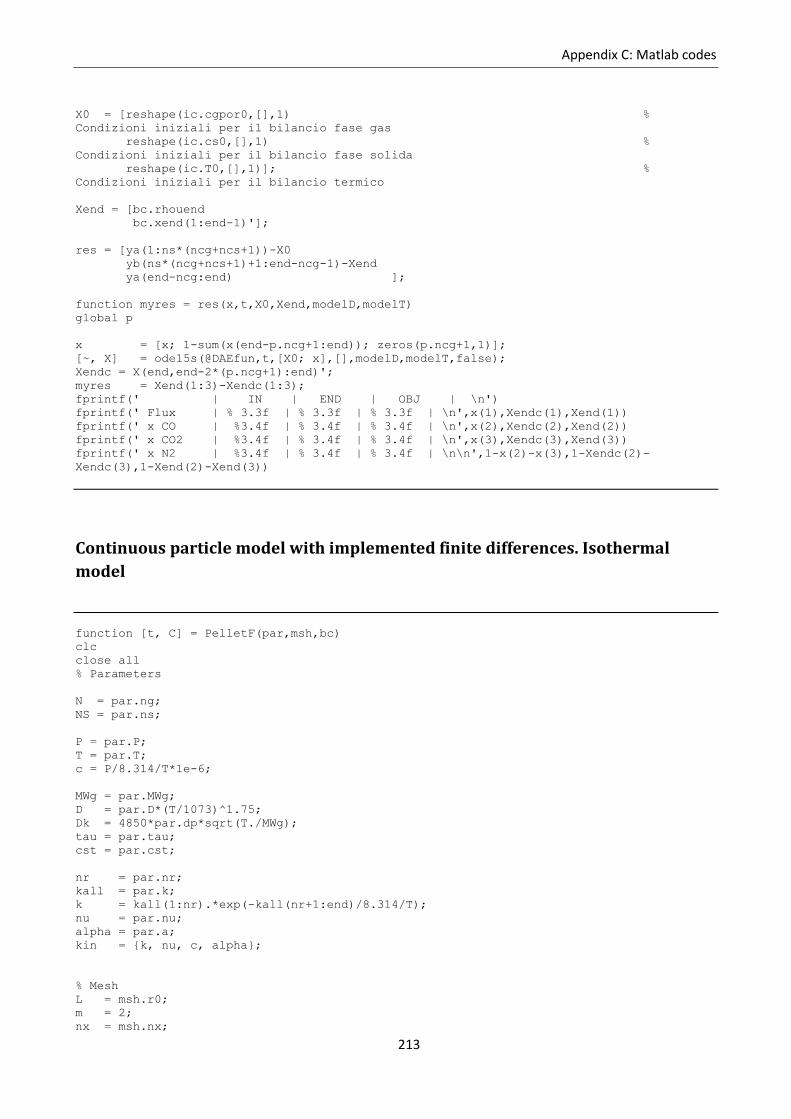
Appendix C: Matlab codes
213
X0 = [reshape(ic.cgpor0,[],1) %
Condizioni iniziali per il bilancio fase gas
reshape(ic.cs0,[],1) %
Condizioni iniziali per il bilancio fase solida
reshape(ic.T0,[],1)]; %
Condizioni iniziali per il bilancio termico
Xend = [bc.rhouend
bc.xend(1:end-1)'];
res = [ya(1:ns*(ncg+ncs+1))-X0
yb(ns*(ncg+ncs+1)+1:end-ncg-1)-Xend
ya(end-ncg:end) ];
function myres = res(x,t,X0,Xend,modelD,modelT)
global p
x = [x; 1-sum(x(end-p.ncg+1:end)); zeros(p.ncg+1,1)];
[~, X] = ode15s(@DAEfun,t,[X0; x],[],modelD,modelT,false);
Xendc = X(end,end-2*(p.ncg+1):end)';
myres = Xend(1:3)-Xendc(1:3);
fprintf(' | IN | END | OBJ | \n')
fprintf(' Flux | % 3.3f | % 3.3f | % 3.3f | \n',x(1),Xendc(1),Xend(1))
fprintf(' x CO | %3.4f | % 3.4f | % 3.4f | \n',x(2),Xendc(2),Xend(2))
fprintf(' x CO2 | %3.4f | % 3.4f | % 3.4f | \n',x(3),Xendc(3),Xend(3))
fprintf(' x N2 | %3.4f | % 3.4f | % 3.4f | \n\n',1-x(2)-x(3),1-Xendc(2)-
Xendc(3),1-Xend(2)-Xend(3))
Continuous particle model with implemented finite differences. Isothermal
model
function [t, C] = PelletF(par,msh,bc)
clc
close all
% Parameters
N = par.ng;
NS = par.ns;
P = par.P;
T = par.T;
c = P/8.314/T*1e-6;
MWg = par.MWg;
D = par.D*(T/1073)^1.75;
Dk = 4850*par.dp*sqrt(T./MWg);
tau = par.tau;
cst = par.cst;
nr = par.nr;
kall = par.k;
k = kall(1:nr).*exp(-kall(nr+1:end)/8.314/T);
nu = par.nu;
alpha = par.a;
kin = {k, nu, c, alpha};
% Mesh
L = msh.r0;
m = 2;
nx = msh.nx;
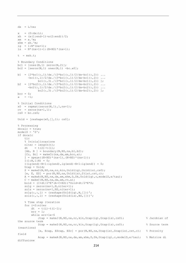
214
dx = L/nx;
x = (0:dx:L);
xh = (x(1:end-1)+x(2:end))/2;
xm = x.^m;
xhm = xh.^m;
ig = 1:N*(nx+1);
is = N*(nx+1)+1:(N+NS)*(nx+1);
t = msh.t;
% Boundary Conditions
bc1 = [ones(N,1) zeros(N,2)];
bc2 = [zeros(N,1) ones(N,1) -bc.x0];
b1 = [2*bc1(:,1)/dx./(3*bc1(:,1)/2/dx-bc1(:,2)) ...
-bc1(:,1)/2/dx./(3*bc1(:,1)/2/dx-bc1(:,2)) ...
bc1(:,3)./(3*bc1(:,1)/2/dx-bc1(:,2)) ];
b2 = [2*bc2(:,1)/dx./(3*bc2(:,1)/2/dx-bc2(:,2)) ...
-bc2(:,1)/2/dx./(3*bc2(:,1)/2/dx-bc2(:,2)) ...
bc2(:,3)./(3*bc2(:,1)/2/dx-bc2(:,2)) ];
bcc = 0;
a = -1;
% Initial Conditions
x0 = repmat(zeros(N,1),1,nx+1);
cv = zeros(nx+1,1);
cs0 = bc.cs0;
Uold = [reshape(x0,[],1); cs0];
% Processing
docalc = true;
modelD = 'S';
if docalc
tic
% Inizializzazione
niter = length(t);
dt = t(2)-t(1);
[Ab, B ] = boundary(N,NS,nx,b1,b2);
[Cc, Bc] = makeCc(nx,dx,xm,bcc,a);
I = speye((N+NS)*(nx+1),(N+NS)*(nx+1));
I(1:N,1:N) = 0;
I(ig(end)-N+1:ig(end),ig(end)-N+1:ig(end)) = 0;
Ucap = Uold;
S = makeS(N,NS,nx,nr,kin,Uold(ig),Uold(is),cs0);
[e, E, ES] = por(N,NS,nx,Uold(is),S(is),cst,c);
A = makeA(N,NS,nx,dx,xm,xhm,D,Dk,Uold(ig),c,modelD,e/tau);
C = makeC(N,NS,nx,dx,xm,cv,a);
bold = (I+dt/2*E*(A-C+ES))*Uold+dt/2*E*S;
solg = zeros(nx+1,N,niter+1);
sols = zeros(nx+1,NS,niter+1);
solg(:,:,1) = (reshape(Uold(ig),N,[]))';
sols(:,:,1) = (reshape(Uold(is),NS,[]))';
% Time step iteration
for i=2:niter
dt = t(i)-t(i-1);
err = 1;
while err>1e-6
Jcap = makeJ(N,NS,nx,nr,kin,Ucap(ig),Ucap(is),cs0); % Jacobian of
the source term
Scap = makeS(N,NS,nx,nr,kin,Ucap(ig),Ucap(is),cs0); % Source term
(reactions)
[e, Ecap, EScap, ESc] = por(N,NS,nx,Ucap(is),Scap(is),cst,c); % Porosity
field
Acap = makeA(N,NS,nx,dx,xm,xhm,D,Dk,Ucap(ig),c,modelD,e/tau); % Matrice di
diffusione
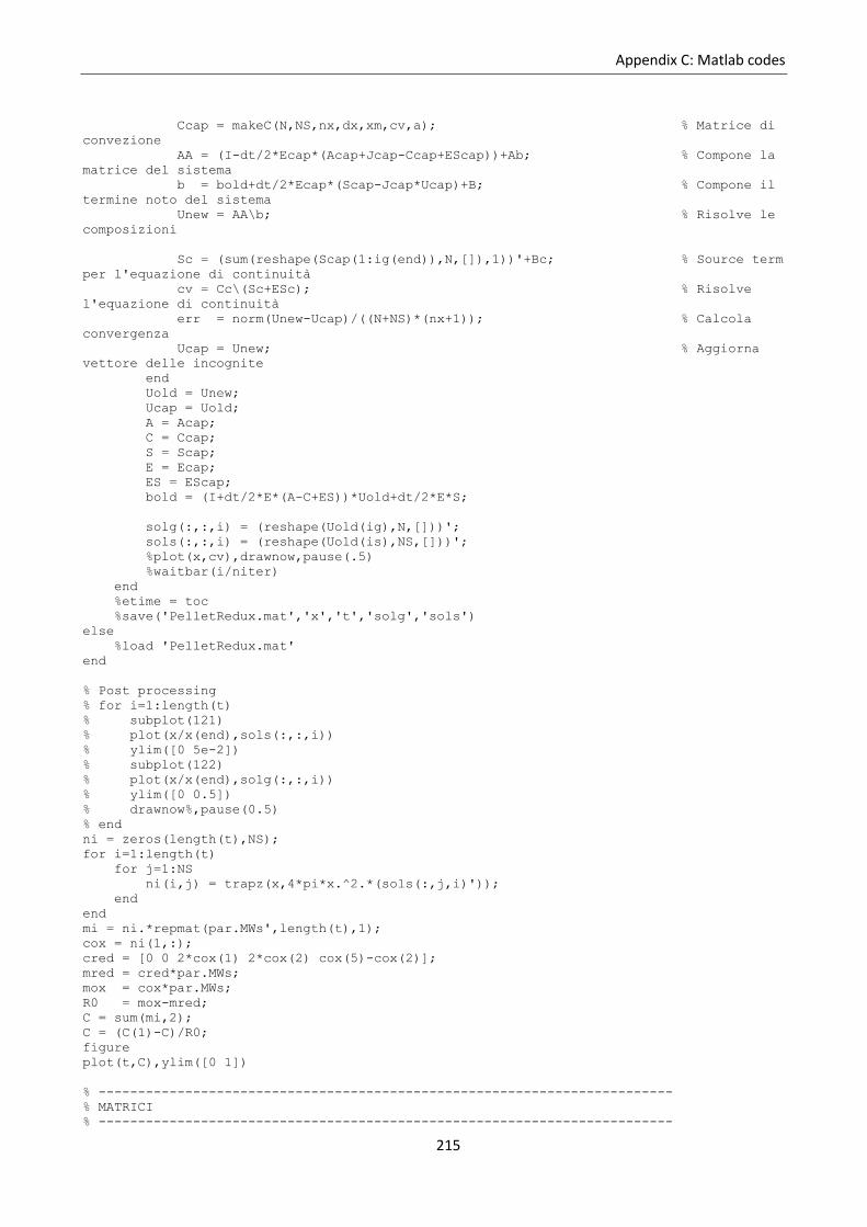
Appendix C: Matlab codes
215
Ccap = makeC(N,NS,nx,dx,xm,cv,a); % Matrice di
convezione
AA = (I-dt/2*Ecap*(Acap+Jcap-Ccap+EScap))+Ab; % Compone la
matrice del sistema
b = bold+dt/2*Ecap*(Scap-Jcap*Ucap)+B; % Compone il
termine noto del sistema
Unew = AA\b; % Risolve le
composizioni
Sc = (sum(reshape(Scap(1:ig(end)),N,[]),1))'+Bc; % Source term
per l'equazione di continuità
cv = Cc\(Sc+ESc); % Risolve
l'equazione di continuità
err = norm(Unew-Ucap)/((N+NS)*(nx+1)); % Calcola
convergenza
Ucap = Unew; % Aggiorna
vettore delle incognite
end
Uold = Unew;
Ucap = Uold;
A = Acap;
C = Ccap;
S = Scap;
E = Ecap;
ES = EScap;
bold = (I+dt/2*E*(A-C+ES))*Uold+dt/2*E*S;
solg(:,:,i) = (reshape(Uold(ig),N,[]))';
sols(:,:,i) = (reshape(Uold(is),NS,[]))';
%plot(x,cv),drawnow,pause(.5)
%waitbar(i/niter)
end
%etime = toc
%save('PelletRedux.mat','x','t','solg','sols')
else
%load 'PelletRedux.mat'
end
% Post processing
% for i=1:length(t)
% subplot(121)
% plot(x/x(end),sols(:,:,i))
% ylim([0 5e-2])
% subplot(122)
% plot(x/x(end),solg(:,:,i))
% ylim([0 0.5])
% drawnow%,pause(0.5)
% end
ni = zeros(length(t),NS);
for i=1:length(t)
for j=1:NS
ni(i,j) = trapz(x,4*pi*x.^2.*(sols(:,j,i)'));
end
end
mi = ni.*repmat(par.MWs',length(t),1);
cox = ni(1,:);
cred = [0 0 2*cox(1) 2*cox(2) cox(5)-cox(2)];
mred = cred*par.MWs;
mox = cox*par.MWs;
R0 = mox-mred;
C = sum(mi,2);
C = (C(1)-C)/R0;
figure
plot(t,C),ylim([0 1])
% -------------------------------------------------------------------------
% MATRICI
% -------------------------------------------------------------------------
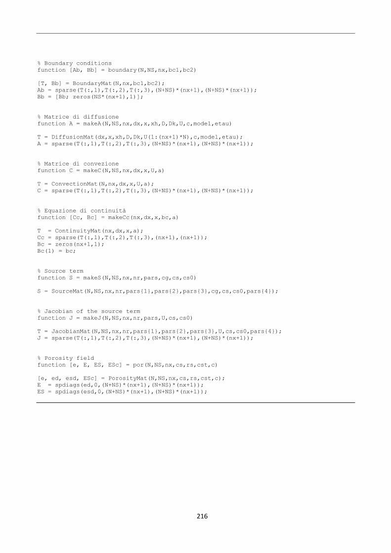
216
% Boundary conditions
function [Ab, Bb] = boundary(N,NS,nx,bc1,bc2)
[T, Bb] = BoundaryMat(N,nx,bc1,bc2);
Ab = sparse(T(:,1),T(:,2),T(:,3),(N+NS)*(nx+1),(N+NS)*(nx+1));
Bb = [Bb; zeros(NS*(nx+1),1)];
% Matrice di diffusione
function A = makeA(N,NS,nx,dx,x,xh,D,Dk,U,c,model,etau)
T = DiffusionMat(dx,x,xh,D,Dk,U(1:(nx+1)*N),c,model,etau);
A = sparse(T(:,1),T(:,2),T(:,3),(N+NS)*(nx+1),(N+NS)*(nx+1));
% Matrice di convezione
function C = makeC(N,NS,nx,dx,x,U,a)
T = ConvectionMat(N,nx,dx,x,U,a);
C = sparse(T(:,1),T(:,2),T(:,3),(N+NS)*(nx+1),(N+NS)*(nx+1));
% Equazione di continuità
function [Cc, Bc] = makeCc(nx,dx,x,bc,a)
T = ContinuityMat(nx,dx,x,a);
Cc = sparse(T(:,1),T(:,2),T(:,3),(nx+1),(nx+1));
Bc = zeros(nx+1,1);
Bc(1) = bc;
% Source term
function S = makeS(N,NS,nx,nr,pars,cg,cs,cs0)
S = SourceMat(N,NS,nx,nr,pars{1},pars{2},pars{3},cg,cs,cs0,pars{4});
% Jacobian of the source term
function J = makeJ(N,NS,nx,nr,pars,U,cs,cs0)
T = JacobianMat(N,NS,nx,nr,pars{1},pars{2},pars{3},U,cs,cs0,pars{4});
J = sparse(T(:,1),T(:,2),T(:,3),(N+NS)*(nx+1),(N+NS)*(nx+1));
% Porosity field
function [e, E, ES, ESc] = por(N,NS,nx,cs,rs,cst,c)
[e, ed, esd, ESc] = PorosityMat(N,NS,nx,cs,rs,cst,c);
E = spdiags(ed,0,(N+NS)*(nx+1),(N+NS)*(nx+1));
ES = spdiags(esd,0,(N+NS)*(nx+1),(N+NS)*(nx+1));
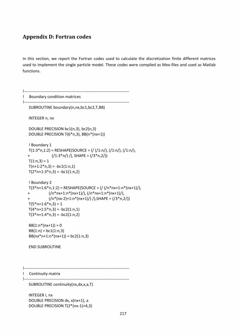
217
Appendix D: Fortran codes
In this section, we report the Fortran codes used to calculate the discretization finite different matrices
used to implement the single particle model. These codes were compiled as Mex-files and used as Matlab
functions.
!------------------------------------------------------------------------------ ! Boundary condition matrices !------------------------------------------------------------------------------ SUBROUTINE boundary(n,nx,bc1,bc2,T,BB) INTEGER n, nx DOUBLE PRECISION bc1(n,3), bc2(n,3) DOUBLE PRECISION T(6*n,3), BB(n*(nx+1)) ! Boundary 1 T(1:3*n,1:2) = RESHAPE(SOURCE = (/ (/1:n/), (/1:n/), (/1:n/), + (/1:3*n/) /), SHAPE = (/3*n,2/)) T(1:n,3) = 1 T(n+1:2*n,3) = -bc1(1:n,1) T(2*n+1:3*n,3) = -bc1(1:n,2) ! Boundary 2 T(3*n+1:6*n,1:2) = RESHAPE(SOURCE = (/ (/n*nx+1:n*(nx+1)/), + (/n*nx+1:n*(nx+1)/), (/n*nx+1:n*(nx+1)/), + (/n*(nx-2)+1:n*(nx+1)/) /),SHAPE = (/3*n,2/)) T(5*n+1:6*n,3) = 1 T(4*n+1:5*n,3) = -bc2(1:n,1) T(3*n+1:4*n,3) = -bc2(1:n,2) BB(1:n*(nx+1)) = 0 BB(1:n) = bc1(1:n,3) BB(nx*n+1:n*(nx+1)) = bc2(1:n,3) END SUBROUTINE !------------------------------------------------------------------------------ ! Continuity matrix !------------------------------------------------------------------------------ SUBROUTINE continuity(nx,dx,x,a,T) INTEGER i, nx DOUBLE PRECISION dx, x(nx+1), a DOUBLE PRECISION T(2*(nx-1)+4,3)
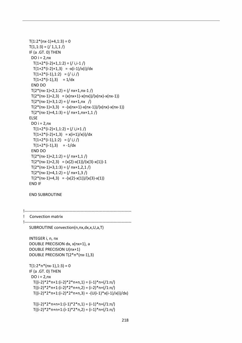
218
T(1:2*(nx-1)+4,1:3) = 0 T(1,1:3) = (/ 1,1,1 /) IF (a .GT. 0) THEN DO i = 2,nx T(1+2*(i-2)+1,1:2) = (/ i,i-1 /) T(1+2*(i-2)+1,3) = -x(i-1)/x(i)/dx T(1+2*(i-1),1:2) = (/ i,i /) T(1+2*(i-1),3) = 1/dx END DO T(2*(nx-1)+2,1:2) = (/ nx+1,nx-1 /) T(2*(nx-1)+2,3) = (x(nx+1)-x(nx))/(x(nx)-x(nx-1)) T(2*(nx-1)+3,1:2) = (/ nx+1,nx /) T(2*(nx-1)+3,3) = -(x(nx+1)-x(nx-1))/(x(nx)-x(nx-1)) T(2*(nx-1)+4,1:3) = (/ nx+1,nx+1,1 /) ELSE DO i = 2,nx T(1+2*(i-2)+1,1:2) = (/ i,i+1 /) T(1+2*(i-2)+1,3) = x(i+1)/x(i)/dx T(1+2*(i-1),1:2) = (/ i,i /) T(1+2*(i-1),3) = -1/dx END DO T(2*(nx-1)+2,1:2) = (/ nx+1,1 /) T(2*(nx-1)+2,3) = (x(2)-x(1))/(x(3)-x(1))-1 T(2*(nx-1)+3,1:3) = (/ nx+1,2,1 /) T(2*(nx-1)+4,1:2) = (/ nx+1,3 /) T(2*(nx-1)+4,3) = -(x(2)-x(1))/(x(3)-x(1)) END IF END SUBROUTINE !------------------------------------------------------------------------------ ! Convection matrix !------------------------------------------------------------------------------ SUBROUTINE convection(n,nx,dx,x,U,a,T) INTEGER i, n, nx DOUBLE PRECISION dx, x(nx+1), a DOUBLE PRECISION U(nx+1) DOUBLE PRECISION T(2*n*(nx-1),3) T(1:2*n*(nx-1),1:3) = 0 IF (a .GT. 0) THEN DO i = 2,nx T((i-2)*2*n+1:(i-2)*2*n+n,1) = (i-1)*n+(/1:n/) T((i-2)*2*n+1:(i-2)*2*n+n,2) = (i-2)*n+(/1:n/) T((i-2)*2*n+1:(i-2)*2*n+n,3) = -(U(i-1)*x(i-1)/x(i)/dx) T((i-2)*2*n+n+1:(i-1)*2*n,1) = (i-1)*n+(/1:n/) T((i-2)*2*n+n+1:(i-1)*2*n,2) = (i-1)*n+(/1:n/)
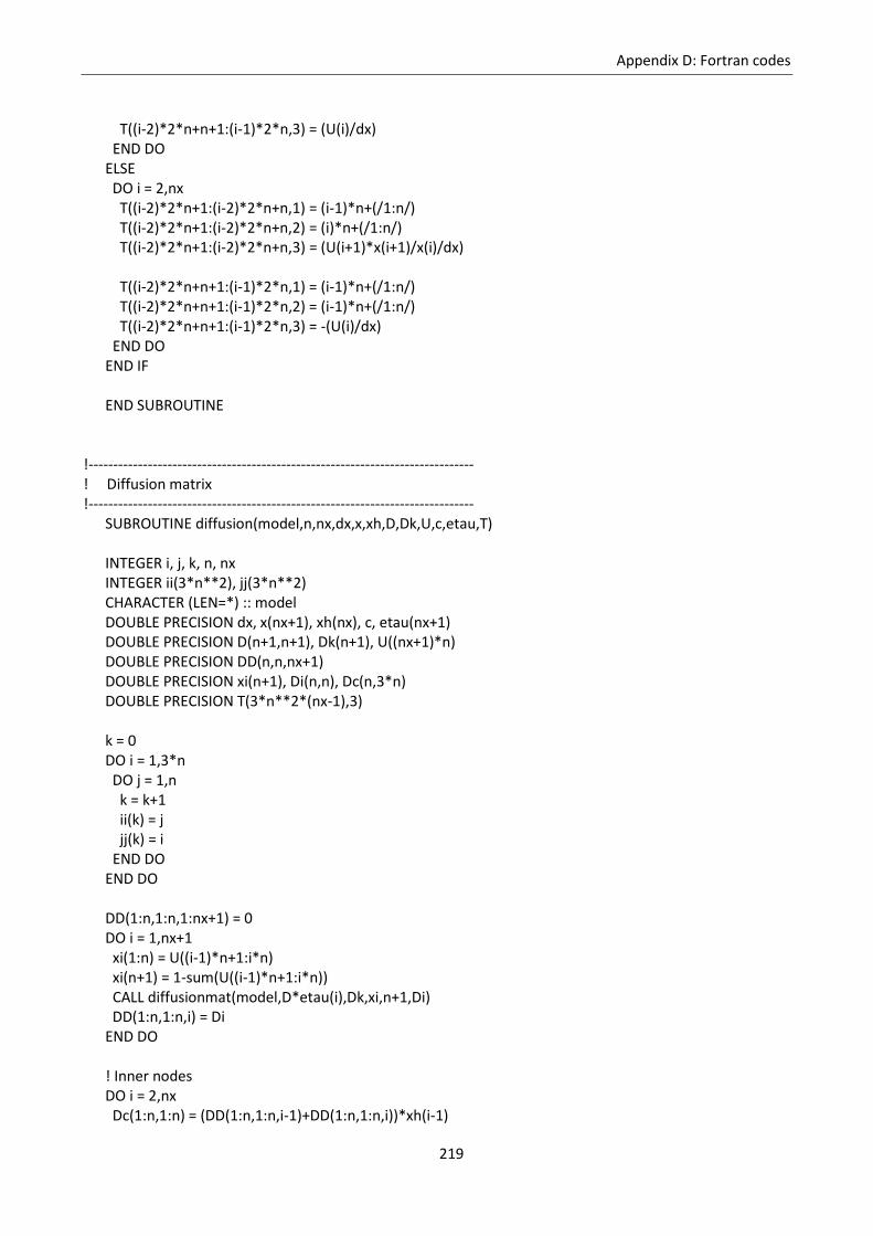
Appendix D: Fortran codes
219
T((i-2)*2*n+n+1:(i-1)*2*n,3) = (U(i)/dx) END DO ELSE DO i = 2,nx T((i-2)*2*n+1:(i-2)*2*n+n,1) = (i-1)*n+(/1:n/) T((i-2)*2*n+1:(i-2)*2*n+n,2) = (i)*n+(/1:n/) T((i-2)*2*n+1:(i-2)*2*n+n,3) = (U(i+1)*x(i+1)/x(i)/dx) T((i-2)*2*n+n+1:(i-1)*2*n,1) = (i-1)*n+(/1:n/) T((i-2)*2*n+n+1:(i-1)*2*n,2) = (i-1)*n+(/1:n/) T((i-2)*2*n+n+1:(i-1)*2*n,3) = -(U(i)/dx) END DO END IF END SUBROUTINE !------------------------------------------------------------------------------ ! Diffusion matrix !------------------------------------------------------------------------------ SUBROUTINE diffusion(model,n,nx,dx,x,xh,D,Dk,U,c,etau,T) INTEGER i, j, k, n, nx INTEGER ii(3*n**2), jj(3*n**2) CHARACTER (LEN=*) :: model DOUBLE PRECISION dx, x(nx+1), xh(nx), c, etau(nx+1) DOUBLE PRECISION D(n+1,n+1), Dk(n+1), U((nx+1)*n) DOUBLE PRECISION DD(n,n,nx+1) DOUBLE PRECISION xi(n+1), Di(n,n), Dc(n,3*n) DOUBLE PRECISION T(3*n**2*(nx-1),3) k = 0 DO i = 1,3*n DO j = 1,n k = k+1 ii(k) = j jj(k) = i END DO END DO DD(1:n,1:n,1:nx+1) = 0 DO i = 1,nx+1 xi(1:n) = U((i-1)*n+1:i*n) xi(n+1) = 1-sum(U((i-1)*n+1:i*n)) CALL diffusionmat(model,D*etau(i),Dk,xi,n+1,Di) DD(1:n,1:n,i) = Di END DO ! Inner nodes DO i = 2,nx Dc(1:n,1:n) = (DD(1:n,1:n,i-1)+DD(1:n,1:n,i))*xh(i-1)
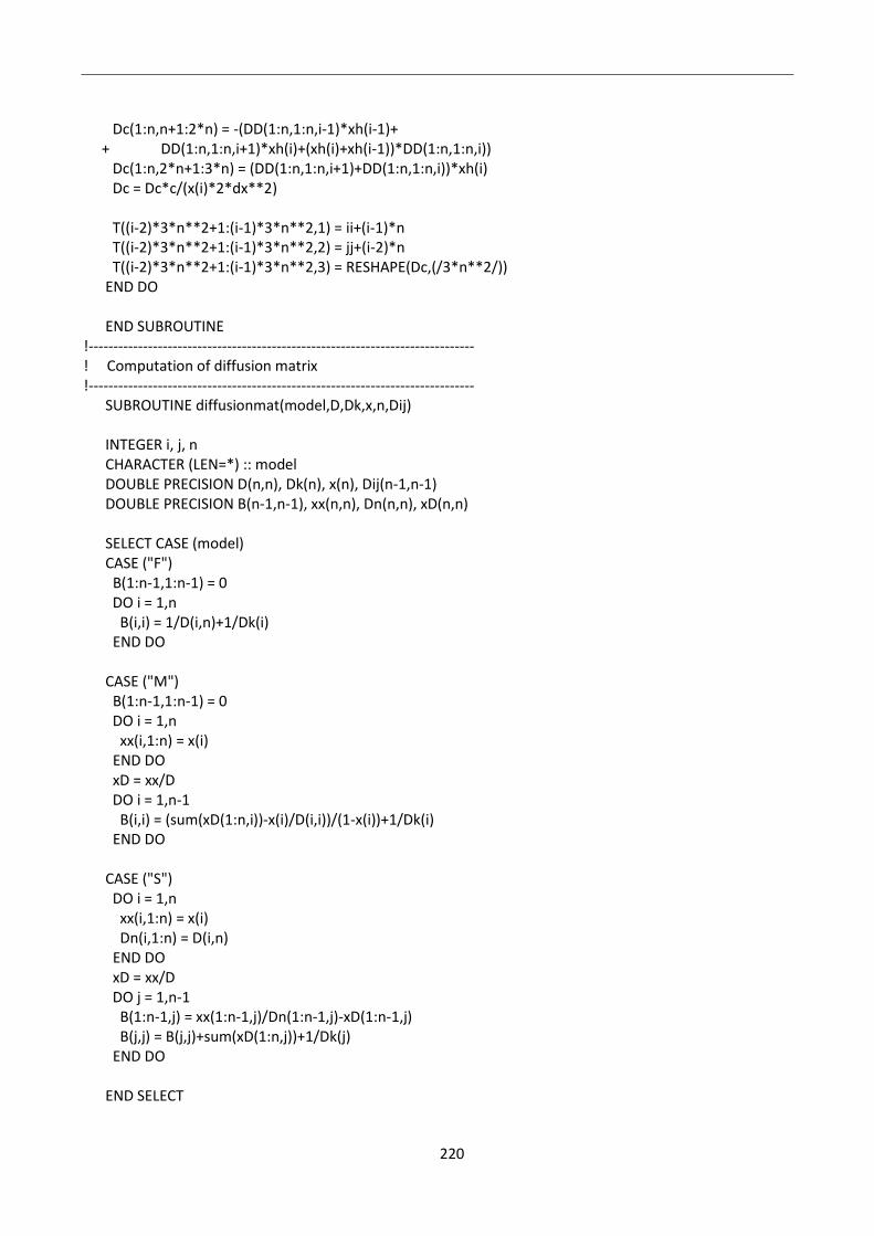
220
Dc(1:n,n+1:2*n) = -(DD(1:n,1:n,i-1)*xh(i-1)+ + DD(1:n,1:n,i+1)*xh(i)+(xh(i)+xh(i-1))*DD(1:n,1:n,i)) Dc(1:n,2*n+1:3*n) = (DD(1:n,1:n,i+1)+DD(1:n,1:n,i))*xh(i) Dc = Dc*c/(x(i)*2*dx**2) T((i-2)*3*n**2+1:(i-1)*3*n**2,1) = ii+(i-1)*n T((i-2)*3*n**2+1:(i-1)*3*n**2,2) = jj+(i-2)*n T((i-2)*3*n**2+1:(i-1)*3*n**2,3) = RESHAPE(Dc,(/3*n**2/)) END DO END SUBROUTINE !------------------------------------------------------------------------------ ! Computation of diffusion matrix !------------------------------------------------------------------------------ SUBROUTINE diffusionmat(model,D,Dk,x,n,Dij) INTEGER i, j, n CHARACTER (LEN=*) :: model DOUBLE PRECISION D(n,n), Dk(n), x(n), Dij(n-1,n-1) DOUBLE PRECISION B(n-1,n-1), xx(n,n), Dn(n,n), xD(n,n) SELECT CASE (model) CASE ("F") B(1:n-1,1:n-1) = 0 DO i = 1,n B(i,i) = 1/D(i,n)+1/Dk(i) END DO CASE ("M") B(1:n-1,1:n-1) = 0 DO i = 1,n xx(i,1:n) = x(i) END DO xD = xx/D DO i = 1,n-1 B(i,i) = (sum(xD(1:n,i))-x(i)/D(i,i))/(1-x(i))+1/Dk(i) END DO CASE ("S") DO i = 1,n xx(i,1:n) = x(i) Dn(i,1:n) = D(i,n) END DO xD = xx/D DO j = 1,n-1 B(1:n-1,j) = xx(1:n-1,j)/Dn(1:n-1,j)-xD(1:n-1,j) B(j,j) = B(j,j)+sum(xD(1:n,j))+1/Dk(j) END DO END SELECT
Appendix D: Fortran codes
221
CALL inversesub(B,n-1,Dij) END SUBROUTINE !------------------------------------------------------------------------------ ! Computation of inverse matrix !------------------------------------------------------------------------------ SUBROUTINE inversesub(A,n,B) INTEGER i, j, n DOUBLE PRECISION A(n,n), B(n,n), Aa(n,2*n) DO i = 1,n DO j = 1,n B(i,j) = 0 END DO B(i,i) = 1 Aa(i,1:n) = A(i,1:n) Aa(i,n+1:2*n) = B(i,1:n) END DO DO j = 1,n-1 DO i = j+1,n IF (Aa(j,j) .NE. 0) THEN Aa(i,1:2*n) = Aa(i,1:n*2)-Aa(i,j)/Aa(j,j)*Aa(j,1:2*n) END IF END DO END DO DO j = n,2,-1 DO i = 1,j-1 IF (Aa(j,j) .NE. 0) THEN Aa(i,1:2*n) = Aa(i,1:n*2)-Aa(i,j)/Aa(j,j)*Aa(j,1:2*n) END IF END DO END DO DO i = 1,n B(i,1:n) = Aa(i,n+1:2*n)/Aa(i,i) END DO END SUBROUTINE !------------------------------------------------------------------------------ ! Reaction rates !------------------------------------------------------------------------------ SUBROUTINE rates(n,ns,nr,k,nu,c,x,cs,cs0,alpha,rp) INTEGER n, ns, nr DOUBLE PRECISION k(nr), nu(n+ns,nr), c, x(n) DOUBLE PRECISION cs(ns), cs0(ns), alpha DOUBLE PRECISION rr(nr), rp(n+ns)
222
rr(1:nr) = 0 IF (cs(1) .GT. 0) THEN rr(1) = k(1)*c*x(1)*(cs(1)/cs0(1))**alpha END IF IF (cs(2) .GT. 0) THEN rr(2) = k(2)*c*x(1)*(cs(2)/cs0(2))**alpha END IF CALL mtimes(nu,rr,(/n+ns,nr/),(/nr,1/),rp) END SUBROUTINE !------------------------------------------------------------------------------ ! Jacobian !------------------------------------------------------------------------------ SUBROUTINE grates(n,ns,nr,k,nu,c,x,cs,cs0,alpha,jrp) INTEGER n, ns, nr DOUBLE PRECISION k(nr), nu(n+ns,nr), c, x(n) DOUBLE PRECISION cs(ns), cs0(ns), alpha DOUBLE PRECISION jrr(nr,n+ns), jrp(n+ns,n+ns) jrr(1:nr,1:n+ns) = 0 IF (cs(1) .GT. 0) THEN jrr(1,1) = k(1)*c*(cs(1)/cs0(1))**alpha jrr(1,n+1) = k(1)*c*x(1)/cs0(1)**alpha*alpha*cs(1)**(alpha-1) END IF IF (cs(2) .GT. 0) THEN jrr(2,1) = k(2)*c*(cs(2)/cs0(2))**alpha jrr(2,n+2) = k(2)*c*x(1)/cs0(2)**alpha*alpha*cs(2)**(alpha-1) END IF CALL mtimes(nu,jrr,(/n+ns,nr/),(/nr,n+ns/),jrp) END SUBROUTINE !------------------------------------------------------------------------------ ! Matrix product !------------------------------------------------------------------------------ SUBROUTINE mtimes(a,b,sa,sb,c) INTEGER sa(2), sb(2), i, j, k DOUBLE PRECISION a(sa(1),sa(2)), b(sb(1),sb(2)), c(sa(1),sb(2)) DO i = 1, sa(1) DO j = 1, sb(2) c(i,j) = 0 DO k = 1, sa(2) c(i,j) = c(i,j) + a(i,k)*b(k,j) END DO
Appendix D: Fortran codes
223
END DO END DO END SUBROUTINE mtimes !------------------------------------------------------------------------------ ! Porosity field !------------------------------------------------------------------------------ SUBROUTINE porosity(n,ns,nx,cs,rs,cst,c,por,E,ES,ESc) INTEGER i, n, ns, nx DOUBLE PRECISION c, cst(ns) DOUBLE PRECISION cs(ns*(nx+1)), rs(ns*(nx+1)) DOUBLE PRECISION por(nx+1), ESc(nx+1), dpordt(nx+1) DOUBLE PRECISION E((n+ns)*(nx+1)), ES((n+ns)*(nx+1)) DOUBLE PRECISION csi(nx+1,ns), rsi(nx+1,ns) DO i = 1,nx+1 csi(i,1:ns) = cs((i-1)*ns+1:i*ns) rsi(i,1:ns) = rs((i-1)*ns+1:i*ns) END DO CALL mtimes(csi,1/cst,(/nx+1,ns/),(/ns,1/),por) CALL mtimes(rsi,1/cst,(/nx+1,ns/),(/ns,1/),dpordt) por = 1-por dpordt = -dpordt E(1:(n+ns)*(nx+1)) = 1 ES(1:(n+ns)*(nx+1)) = 0 ESc(1:nx+1) = 0 DO i = 2,nx E((i-1)*n+1:i*n) = 1/(c*por(i)) ES((i-1)*n+1:i*n) = -c*dpordt(i) END DO ESc(2:nx) = -c*dpordt(2:nx) END SUBROUTINE !------------------------------------------------------------------------------ ! Source vector !------------------------------------------------------------------------------ SUBROUTINE source(n,ns,nx,nr,k,nu,c,x,cs,cs0,alpha,S) INTEGER i, n, ns, nx, nr DOUBLE PRECISION k(nr), nu(n+ns,nr), c, x(n*(nx+1)) DOUBLE PRECISION cs(ns*(nx+1)), cs0(ns*(nx+1)), alpha DOUBLE PRECISION rp(n+ns), S((n+ns)*(nx+1)) S(1:(n+ns)*(nx+1)) = 0
224
DO i = 1,nx+1 CALL rates(n,ns,nr,k,nu,c,x((i-1)*n+1:i*n), + cs((i-1)*ns+1:i*ns),cs0((i-1)*ns+1:i*ns),alpha,rp) IF ((i .NE. 1) .AND. (i .NE. nx+1)) THEN S((i-1)*n+1:i*n) = rp(1:n) END IF S(n*(nx+1)+(i-1)*ns+1:n*(nx+1)+i*ns) = rp(n+1:n+ns) END DO END SUBROUTINE !------------------------------------------------------------------------------ ! Jacobian matrix !------------------------------------------------------------------------------ SUBROUTINE jacobian(n,ns,nx,nr,k,nu,c,x,cs,cs0,alpha,T) INTEGER i, j, l, m, n, ns, nx, nr DOUBLE PRECISION k(nr), nu(n,nr), c, x(n*(nx+1)) DOUBLE PRECISION cs(ns*(nx+1)), cs0(ns*(nx+1)), alpha DOUBLE PRECISION ij(n+ns), jrp(n+ns,n+ns) DOUBLE PRECISION T((n+ns)**2*(nx+1)-2*n*(n+ns),3) m = 0 T(1:(n+ns)**2*(nx+1)-2*n*(n+ns),1:3) = 0 DO l = 1,nx+1 ij = (/ (l-1)*n+1:l*n, n*(nx+1)+(l-1)*ns+1:n*(nx+1)+l*ns /) CALL grates(n,ns,nr,k,nu,c,x((l-1)*n+1:l*n), + cs((l-1)*ns+1:l*ns),cs0((l-1)*ns+1:l*ns),alpha,jrp) DO i = 1,n+ns IF (((l .NE. 1) .AND. (l .NE. nx+1)) .OR. (i .GT. n)) THEN DO j = 1,n+ns m = m+1 T(m,1:3) = (/ ij(i), ij(j), jrp(i,j) /) END DO END IF END DO END DO END SUBROUTINE
225
References
[1] J. Szekely, J. W. Evans, and H. Y. Sohn, Gas solid reactions: Academic Press, 1976. [2] P. A. Ramachandran and L. K. Doiraiswamy, "Modeling of Noncatalytic Gas-Solid Reactions," AIChE
J., vol. 28, pp. 881-900, 2004. [3] Y. C. Wen, "Noncatalytic heterogeneous solid fluid reaction models," Ind. Eng. Chem., vol. 60, pp.
34-54, 1968. [4] S. P. Trushenski, K. Li, and W. O. Philbrook, "Non-Topochemical reduction of iron oxides," Metall.
Trans., vol. 5, pp. 1149-1158, 1974. [5] S. K. Bhatia and D. D. Perlmutter, "A random pore model for fluid-fluid reactions, I: isothermal,
kinetic control," AIChE J., vol. 26, pp. 379-386, 1980. [6] A. K. Sadhukhan, P. Gupta, and R. K. Saha, "Characterization of porous structure of coal char from a
single devolatilized coal particle: Coal combustion in a fluidized bed," Fuel Proc. Tech., vol. 90, pp. 692-700, 2009.
[7] A. Gomez-Barea and P. Ollero, "An approximae method for solving gas-solid non-catalytic reactions," Chem. Eng. Sci., vol. 61, pp. 3725-3735, 2006.
[8] F. Patisson, M. G. Francois, and D. Ablitzer, "A non-isothermal, non-equimolar transient kinetic model for gas-solid reactions," Chem. Eng. Sci., vol. 53, pp. 697-708, 1998.
[9] M. S. Valipour and Y. Saboohi, "Modeling of multiple noncatalytic gas-solid reactions in a moving bed of porous pellets based on finite volume method," Heat Mass Transfer, vol. 43, pp. 881-894, 2007.
[10] J. Szekely and J. W. Evans, "Studies in gas–solid reactions: part I. A structural model for the reaction of porous oxides with a reducing gas," Metall. Trans. 2, pp. 1691–1711, 1971.
[11] L. D. Schmidt, The Eingineering of Chemical Reactions. New York: Oxford University Press, 1998. [12] S. Yagi and D. Kunii, "Studies on combustion of carbon particles in flames and fluidized beds," The
5th symposium on combustion, vol. New York, USA, pp. 231-236, 1955. [13] A. Abad, J. Adanez, A. Cuadrat, F. Garcia-Labiano, P. Gayan, and L. F. de Diego, "Kinetics of redox
reactions of ilmenite for chemical-looping combustion," Chem. Eng. Sci., vol. 66, pp. 689-702, 2011. [14] A. Amiri, G. D. Ingram, A. V. Bekker, I. Livk, and N. E. Maynard, "A multi-stage, multi-reaction
shrinking core model for self-inhibiting gas-solid reactions," Adv. Powder Technol., vol. 24, pp. 728-736, 2013.
[15] P. K. Gbor and C. Q. Jia, "Critical evaluation of coupling particle size distribution with the shrinking core model," Chem. Eng. Sci., vol. 59, pp. 1979-1987, 2004.
[16] H. Kruggel-Emden, S. Rickelt, F. Stepanek, and M. A., "Development and testing of an interconnected multiphase CFD-model for chemical looping combustion," Chem. Eng. Sci., vol. 65, pp. 4732-4745, 2010.
[17] H. Kruggel-Emden, F. Stepanek, and M. A., "A study on the role of reaction modeling in Multi-phase CFD-based simulations of Chemical Looping Combustion," Oil Gas Sci. Tech., vol. 66, pp. 313-331, 2011.
[18] D. R. Parisi and M. A. Laborde, "Modeling of counter current moving bed gas-solid reactor used in direct reduction of iron ore," Chem. Eng. J., vol. 104, pp. 35-43, 2004.
[19] E. D. Negri, O. M. Alfano, and M. G. Chiovetta, "Direct Reduction of Hematite in a Moving-Bed Reactor. Analysis of the Water Gas Shift Reaction Effects on the Reactor Behavior," Ind. Eng. Chem. Res., vol. 30, pp. 474-482, 1991.
[20] M. Ohmi and T. Usui, "Improved theory on the rate of reduction of single particles and fixed beds of iron oxide pellets with hydrogen," Trans. ISIJ, vol. 22, pp. 66-74, 1982.
226
[21] Y. Hara, M. Tsuchiya, and S. Kondo, "Intraparticle temperature of iron-oxide pellet during the reduction," Tetsu-to-Hagane, vol. 60, pp. 1261-1270, 1974.
[22] Comsol Multiphysics v4.2, COMSOL Inc. www.comsol.com [Online]. Available: www.comsol.com [23] MathWorks MATLAB R2011a www.mathworks.com [Online]. [24] D. Dalle Nogare, A. Zugliano, A. Primavera, T. Melchiori, and P. Canu, "Multiphysics simulation of a
DRP shaft furnace," Proc. Steelsim2013, 2013. [25] R. Artoni, A. Zugliano, A. Primavera, P. Canu, and A. Santomaso, "Simulation of dense granular
flows: comparison with experiments," Chem. Eng. Sci., vol. 66, pp. 548-557, 2011. [26] H. Yamaoka and Y. Kamei, "A three dimensional mathematical simulation model of shaft type
reduction furnace and cupola type melting furnace," Tetsu-to-Hagané, vol. 74, pp. 2254–2261, 1988.
[27] J. Xu, S. Wu, M. Kou, and K. Du, "Numerical analysis of the characteristics inside pre-reduction shaft furnace and its operation parameters optimization by using a three-dimensional full scale mathematical model," ISIJ Intern., vol. 53, pp. 576–582, 2013.
[28] N. Towhidi and J. Szekely, "The influence of carbon deposition of the reduction kinetics of commercial grade hematite pellets with CO, H2 and N2," Metall. Trans. B, vol. 148, pp. 359–366, 1983.
[29] Q. T. Tsay, W. H. Ray, and J. Szekely, "The modeling of hematite reduction with hydrogen plus carbon monoxide mixtures. Part I: the behavior of single pellets," AIChE J., vol. 22, pp. 1064-1072, 1976.
[30] Q. T. Tsay, R. W.H., and S. J., "The modeling of hematite reduction with hydrogen plus carbon monoxide mixtures: Part II. The direct reduction process in shaft furnace arrangement," AIChE J., vol. 22, pp. 1072–1079, 1976.
[31] Y. Shigeno, T. Sakakibara, and Y. Omori, "In situ measurement of effective gas diffusivity through hematite pellets during stepwise reductions," Metall. trans. B, pp. 677–687, 1990.
[32] GRImech3.0, Gas Research Institute, Berkeley Mechanical Engineering Dept. www.me.berkeley.edu/grimech/ [Online].
[33] R. B. Bird, W. E. Stewart, and E. N. Lightfoot, Transport phenomena, 2nd edition ed.: Wiley, 2002. [34] R. Taylor and R. Krishna, Multicomponent mass transfer: Wiley, 1993. [35] G. Salejova, Z. Grofa, O. Solcovab, P. Schneiderb, and J. Koseka, "Strategy for predicting effective
transport properties of complex porous structures," Comp. Chem. Eng., vol. 35, pp. 200-211, 2011. [36] F. J. Valdes-Parada and J. Alvarez-Ramirez, "On the effective diffusivity under chemical reaction in
porous media," Chem. Eng. Sci., vol. 65, pp. 4100-4104, 2010. [37] A. Abad, F. Garcıia-Labiano, L. de Diego, P. Gayan, and J. Adanez, "Reduction kinetics of Cu-, Ni-,
and Fe-based oxygen carriers using syngas (CO + H2) for Chemical-Looping Combustion," Energy Fuels, vol. 21, pp. 1843-1853, 2007.
[38] A. Rubel, K. Liu, J. Neathery, and D. Taulbee, "Oxygen carriers for chemical looping combustion of solid fuels," Fuel, vol. 88, pp. 876-884, 2009.
[39] H. Jin and M. Ishida, "Reactivity study on a novel hydrogen fueled chemical looping combustion," Int. J. Hydr. Energy vol. 26, pp. 889-894, 2001.
[40] P. Erri and A. Varma, "Diffusional effects in nickel oxide reduction kinetics," Ind. Eng. Chem. Res., vol. 48, pp. 4-6, 2009.
[41] S. Roux, A. Bensakhria, and G. Antonini, "Study and improvement of the regeneration of metallic oxides used as oxygen carriers for a new combustion process," Int. J. Chem. React. Eng., vol. 4, p. A38, 2006.
[42] H. Tian, K. Chaudhari, T. Simonyi, J. Poston, T. Liu, T. Sanders, G. Veser, and R. Siriwardane, "Chemical-looping combustion of coal-derived synthesis gas over copper oxide oxygen carriers," Energy Fuels, vol. 22, pp. 3744-3755, 2008.
[43] L. F. de Diego, F. García-Labiano, J. Adánez, P. Gayán, A. Abad, and B. M. e. a. Corbella, "Development of Cu-based oxygen carriers for chemical-looping combustion," Fuel, vol. 83, pp. 1749-1757, 2004.
References
227
[44] Q. Zafar, T. Mattisson, and B. Gevert, "Redox investigation of some oxides of transition-state metals Ni, Cu, Fe, and Mn supported on SiO2 and MgAl2O4," Energy Fuels, vol. 20, pp. 34-44, 2006.
[45] H. Leion, T. Mattisson, and A. Lyngfelt, "Use of ores and industrial products as oxygen carriers in chemical-looping combustion," Energy Fuels, vol. 23, pp. 2307-2315, 2009.
[46] H. Leion, A. Lyngfelt, M. Johansson, E. Jerndal, and T. Mattisson, "The use of ilmenite as an oxygen carrier in chemical-looping combustion," Chem. Eng. Res. Des., vol. 86, pp. 1017-1026, 2008.
[47] J. Adanez, A. Cuadrat, A. Abad, P. Gayan, L. F. de Diego, and F. Garcia-Labiano, "Ilmenite activation during consecutive redox cycles in Chemical-Looping Combustion," Energy Fuels, vol. 24, pp. 1402-1413, 2010.
[48] D. Bhogeswara Rao and M. Rigaud, "Kinetics of the oxidation of Ilmenite," Oxid. Metals, vol. 9, pp. 99-116, 1975.
[49] M. M. Azis, E. Jerndal, H. Leion, T. Mattisson, and A. Lyngfelt, "On the evaluation of synthetic and natural ilmenite using syngas as fuel in chemical-looping combustion (CLC)," Chem. Eng. Res. Des., vol. 88, pp. 1505-1514, 2010.
[50] S. Noorman, F. Gallucci, M. Van SintAnnaland, and J. A. M. Kuipers, "A theoretical investigation of CLC in packed beds. Part 1: Particle model," Chem. Eng. J., vol. 167, pp. 297-307, 2011.
[51] Z. Zhou, L. Han, and G. M. Bollas, "Model-based analysis of bench-scale fixed-bed units for chemical-looping combustion," Chem. Eng. J., vol. 233, pp. 331-348, 2013.
[52] L. Han, Z. Zhou, and G. M. Bollas, "Heterogeneous modeling of chemical-looping combustion. Part1: Reactor model," Chem. Eng. Sci., vol. 104, pp. 233-249, 2013.
[53] S. Sotirchos and H. Yu, "Mathematical modelling of gas-solid reactions with solid product," Chem. Eng. Sci., vol. 40, pp. 2039-2052, 1985.
[54] K. Dam-Johansen, P. Hansen, and K. Ostergaard, "High temperature reaction between sulphur dioxide and limestone- III. A grain-micrograin model and its verification," Chem. Eng. Sci., vol. 46, pp. 847-853, 1991.
[55] P. den Hoed and A. Luckos, "Oxidation and reduction of Iron-Titanium oxides in Chemical Looping Combustion: A phase-chemical description," Oil Gas Sci. Technol., vol. 66, pp. 249-263, 2011.
[56] G. Boole, A treatise on the calculus of finite differences, 2nd ed.: Macmillan and Company, 1872. [57] J. Cranck and P. Nicolson, "A practical method for numerical evaluation of solutions of partial
differential equations of the heat conduction type," Proc. Camb. Phil. Soc., vol. 43, pp. 50-67, 1947. [58] A. Niksiar and A. Rahimi, "A study on deviation of noncatalytic gas–solid reaction models due to
heat effects and changing of solid structure," Powder Technol., vol. 193, pp. 101-109, 2009. [59] F. Patisson and D. Ablitzer, "Physicochemical and thermal modelling of the reaction between a
porous pellet and a gas," Powder Technol., vol. 128, pp. 300-305, 2002. [60] A. K. Sadhukhan, P. Gupta, and R. K. Saha, "Modelling of combustion characteristics of high ash coal
char particles at high pressure: Shrinking reactive core model," Fuel, vol. 89, pp. 162-169, 2010. [61] O. Levenspiel, Chemical Reaction Engineering, 3rd edition: John Wiley and Sons, 1999. [62] M. Ishida and C. Y. Wen, "Comparison of zone-reaction model and unreacted-core shrinking model
in solid-gas reactions - I Isothermal analysis," Chem. Eng. Sci., vol. 26, pp. 1031-1041, 1971. [63] D. D. Do, "On the validity of the shrinking core model in non catalytic gas solid reaction," Chem.
Eng. Sci., vol. 37, pp. 1477-1481, 1982. [64] T. Melchiori and P. Canu, "Improving the quantitative description of reacting porous solids: critical
analysys of the shrinking core model by comparison to the generalized grain model," Ind. Eng. Chem. Res., accepted, in press.
[65] J. Villadsen and M. L. Michelsen, Solution of differential equation models by polynomial approximation: Prentice-Hall, 1978.
[66] A. Afshar Ebrahimi, H. Ale Ebrahim, and E. Jamshidi, "Solving partial differential equations of gas–solid reactions by orthogonal collocation," Comp. Chem. Eng., vol. 32, pp. 1746-1759, 2008.

228
References
229
Acknowledgements
I would like to thank prof. Martin van Sint Annaland and prof. Fausto Gallucci, who hosted me in the
Multiphase Reactors research group at TU/e for eight months, and gave me the opportunity to improve my
research activity. Many thanks to all the people from SMR group, particularly to Maria for her support on
the experimental part. I would also like to mention Luca, Arash, Lucia, Valentina, José, and all the other
friends that I met in Eindhoven.
Ringraziamenti
Vorrei fare un grosso ringraziamento al mio relatore, prof. Paolo Canu, per tutto quanto fatto per me in
questi anni, e con cui posso dire di aver trovato un bellissimo rapporto. Grazie a lui ho scelto la strada del
dottorato, e con il senno di poi gli sono molto riconoscente per avermi spinto in questa direzione. Da lui ho
imparato moltissimo, non solo a livello della ricerca in sé ma anche per quanto riguarda tutto il mondo che
le sta attorno. Insomma è stato per me molto più che una guida. Un ringraziamento particolare a Nicola,
che ha trasformato l'atmosfera del nostro gruppo di ricerca rendendola fantastica, dentro e fuori le mura
dell'Università. Vorrei anche ringraziare Alberto e Micol, e tutti i ragazzi tesisti che ho conosciuto purtroppo
solo nell'ultimo anno, con cui abbiamo condiviso quest'ultimo periodo assieme. Non da ultimo, vorrei
ringraziare la mia famiglia per tutto il supporto datomi in questi anni, e per avermi sostenuto in ogni mia
scelta che ho fatto fino ad ora. Infine un grandissimo grazie al mio gruppo di amici storici, in particolare Pip,
Leo e Nick, e tutti gli altri per cui la vita ha voluto che le nostre strade si separassero nel tempo. A tutte le
persone che mi sono care, e che ora sto per lasciare, va un forte abbraccio di affetto e riconoscenza.