UNIVERSITA’ DEGLI STUDI DI PADOVA

DIPARTIMENTO DI SCIENZE ECONOMICHE E AZIENDALI

“MARCO FANNO”

CORSO DI LAUREA MAGISTRALE IN ECONOMIA INTERNAZIONALE

LM-56 Classe delle lauree magistrali in SCIENZE DELL’ECONOMIA

Tesi di laurea

Una visione d’insieme dell’ipotesi di Efficienza di Mercato INDAGINE SULL’EMH & SUL MERCATO ITALIANO

An Overall View Of The Efficient Market Hypothesis INVESTIGATION ON THE EMH & ON THE ITALIAN MARKET

Relatore:

Prof. FONTINI FULVIO

Correlatore:

Prof. CAPORIN MASSIMILIANO

Laureando:

FUIANO FRANCESCO

Anno Accademico 2014-2015

1

Il candidato dichiara che il presente lavoro è originale e non è già stato sottoposto, in tutto o in

parte, per il conseguimento di un titolo accademico in altre Università italiane o straniere.

Il candidato dichiara altresì che tutti i materiali utilizzati durante la preparazione

dell’elaborato sono stati indicati nel testo e nella sezione “Riferimenti bibliografici” e che le

eventuali citazioni testuali sono individuabili attraverso l’esplicito richiamo alla pubblicazione

originale.

Firma dello studente

_________________

2

“In God we trust, all others must bring data”

Edwards Deming

3

Alla mia famiglia che mi ha accompagnato lungo questo percorso

4

Abstract .............................................................................................................................................. 6

Introduction ....................................................................................................................................... 7

1. The Efficient Market Hypothesis. ................................................................................................ 7

1.1 The EMH since the beginning .................................................................................................... 7

1.2 Critics and hints on Behavioural Finance ............................................................................... 16

2. Test on the EMH ......................................................................................................................... 18

2.1. An historical review ................................................................................................................. 18

2.2. Previous studies: the Italian cases ........................................................................................... 24

2.2.1 The Weak-form ........................................................................................................................ 24

2.2.1 The Semi-strong-form ............................................................................................................. 25

2.2.2 A continuing process .............................................................................................................. 26

3. Anomalies on the EMH ............................................................................................................... 28

3.1 Calendar Anomalies .................................................................................................................. 28

3.2 The week-end effect ................................................................................................................... 29

3.2.1 Other calendar anomalies ......................................................................................................... 31

3.3 Fundamental Anomalies ........................................................................................................... 34

3.4 The P/E effect ............................................................................................................................. 34

3.4.1 Other fundamental anomalies ................................................................................................... 36

3.5. Technical Anomalies ................................................................................................................ 36

3.5.1 Hints on technical anomalies .................................................................................................... 36

3.6. Do famous anomalies persist nowadays? ............................................................................... 37

3.7. How many ways to test the EMH? .......................................................................................... 38

3.7.1 Hints on different ways to test the EMH and the anomalies affecting it: Fundamental and

Technical analysis. ............................................................................................................................ 38

4. Is the Italian market efficient? ................................................................................................... 39

4.1 Testing the EMH on the Italian Market .................................................................................. 40

Index Analysis .................................................................................................................................. 40

4.1.1 Data .......................................................................................................................................... 40

4.1.2 Weak Hypothesis...................................................................................................................... 47

4.1.3 Methodology and Results ......................................................................................................... 47

Companies Analysis ........................................................................................................................ 62

4.1.4 Data .......................................................................................................................................... 63

4.1.5 Weak Hypothesis...................................................................................................................... 70

4.1.6 Methodology and Results ......................................................................................................... 71

5

4.1.7 Semi-Strong Hypothesis ........................................................................................................... 92

5. The ways we access the market .................................................................................................. 98

5.1 Exchange-Traded Funds ........................................................................................................... 98

5.2 Testing the weak form of EMH through the Exchange-traded Funds in Italy ................... 99

5.3 Weak Hypothesis ...................................................................................................................... 103

5.4 Data ........................................................................................................................................... 104

5.5 Methodology and Results .......................................................................................................... 104

Conclusions .................................................................................................................................... 121

References ...................................................................................................................................... 124

6

Abstract

Il presente lavoro è stato sviluppato col proposito di esaminare l’ipotesi di efficienza di

mercato definita da Eugene Fama. Dopo un’analisi preliminare volta a comprendere le tappe

principali che hanno portato alla definizione dell’ipotesi, si è proceduto con un’osservazione

relativa alle critiche poste in essere a partire dagli anni ’70 contro la tesi di efficienza

informativa. Quindi dopo una panoramica più approfondita delle anomalie rilevate negli anni

nel mercato, si è proceduto con un’analisi empirica del mercato volta a verificare la presenza

di efficienza debole e semi-forte, oltre la presenza di possibili anomalie. Oggetto dell’analisi

sono stati i sei indici principali della Borsa Italiana ed un campione di società estratto dal

FTSE MIB. Inoltre, dopo una definizione approfondita del loro ruolo nel mercato, si è

proceduto ad esaminare l’efficienza nel mercato degli ETF italiani, per verificare se le loro

caratteristiche li rendono più funzionali ad un mercato efficiente.

7

Introduction

The present work has been developed with the aim to explain the complexity over the concept

of the Efficient Market Hypothesis (EMH). First, the analysis focuses on the literature relative

to the hypothesis since its origin with the Eugene Fama’s work. From here onward the

attention is on the dualism between the criticism against the concept and the awareness that

the hypothesis seems legit. Many detailed works follow one another over the time; that

implies an evolution of the concept and its estimation methods. The Technical Analysis, the

Fundamental analysis and the Behavioural Finance are the most representatives theoretical

argumentations in net contrast with the EMH.

The step forward is to empirically analyse the efficiency for the Italian case, underlying some

unsolved aspects such as the anomalies of the market. These second part of our investigation

starts with the examination of empirical worldwide evidences during years until the latest

ones. Concurrently with this examination, this work presents its own empirical evidence on

the Italian case.

These investigations concern the different levels of the EMH, dividing the weak hypothesis

from the semi-strong one.

A multitude of methods used over time in the search for efficiency comes up. The analysis

ends up with some consideration about the truthfulness of the EMH, showing the results

among the various Italian markets, best considering the Exchange-Traded Funds.

1. The Efficient Market Hypothesis.

1.1 The EMH since the beginning

Despite the existence of a certain documentation dated back to the eighteenth century, the first

evidence about the concept of Efficient Market Hypothesis was given by Louis Bachelier. In

1900 Bachelier developed the groundwork for the hypothesis considered: first, modelling the

mathematics of the Brownian motion, and then, introducing the formulation for a Random

walk in security prices. He was the first to provide the law of probability for stock market

fluctuations: starting from the total mathematical expectation of a player (sum of the possible

gains weighted with their relative probabilities of realization), he found out that the

expectation of the speculator was zero. Indeed he stated that past, present, and even future

events were reflected by market price, but at the same time, they did not seem to influence

price changes. Bachelier developed this analysis assuming that stock returns follow a fair

game, that the probability that the future price 𝑝𝑡+𝑛 is a function of the current one (𝑝𝑡) and

8

that transactions are uniformly spread across time (finite variance of the distribution of price

changes and large transaction number during the given lapse of time). Bachelier’s

argumentation leads to the Markov-dependence as well as the utilization of the Central Limit

theorem to call upon Normality. The consequence is the fact that the conditional and

unconditional probability of the future price at the future time is governed by the Gaussian

Law and proportional to the square root of time.1

Unfortunately, his works passed unnoticed because of the backwardness of his time. Moving

forward on the historical evolution of the efficient market concept, we find Wesley Mitchell.

He was the first to discover that the distributions of price changes cannot be associated to

samples from Gaussian populations. Even John Maynard Keynes, in 1923, stated that

investors gained because of the risk bearing and not because they were able to predict better

than the market what the future would show them. He confirmed his statement in 1936,

comparing the stock market with a beauty contest and claiming that investors’ decisions were

the results of their animal spirits. It is a duty to mention Holbrook Working too. He equated

stock returns to numbers from a lottery.

Early, Cowles concluded that there were no evidences of the possibility to predict the market.

However, in 1937, he found evidences of serial correlation in averaged time series indices of

stock prices, as long as he reported again that investment professionals do not beat the market

in 1944. An important contribute to the Efficient Market Hypothesis was pointed out by

Milton Friedman in 1953. Friedman stated that the efficient market held also when trading

strategies of investors were correlated; these could happen because of the arbitrage. In the

same year, Kendall, examined 22 UK stock and commodity price series discovering they were

basically random. Moreover he found out the time dependence of the empirical variance (the

non-stationarity). In 1959, after Kendal’s contribute, Harry Roberts showed that a random

walk and the current stock series resembled themselves.

Lingering on these last two authors, it is possible to summarise the literature point of view of

this first studying period of the efficient market. Hence, the random walk formulation was

seen as a system that generates the stock price process as follow:

𝑝𝑡 = 𝑝𝑡−1 + 𝑟𝑡, 𝑡 ∈ 𝑇 (1)

Random sample model (or chance mechanism)

1 History of the Efficient Market Hypothesis, Martin Sewell, 2011, UCL Department of Computer Science

9

Where 𝑟𝑡~𝐼𝐼𝐷(0, 𝜎2), that is 𝑟𝑡 is an Independent and Identically Distributed process with zero

mean and constant variance 𝜎2. Here prices are assumed to be the partial sum of returns,

𝑝𝑡 = ∑ 𝑟𝑘𝑡𝑘=1 , 𝑡 ∈ 𝑇.

The issues of this former configuration is both on the absence of explicit distributional

assumption and the fact that {𝑝𝑡 , 𝑡 ∈ 𝑇} implies that the first two moments exist (Markov-

dependent process2). Nevertheless this literature implicitly hid that the distribution of returns

was Normal and so the random walk as well. This means that 𝑟𝑡~𝑁𝐼𝐼𝐷(0, 𝜎2) is a Normal

Independent and Identically Distributed process (with N stands for Normality).

For this model the process {𝑝𝑡 , 𝑡 ∈ 𝑇} is Markov-dependent with a probabilistic structure

given by:

(𝑝𝑡

𝑝𝑡−1) ~𝑁 [(

00

) , (𝜎2𝑡 𝜎2(𝑡 − 1)

𝜎2(𝑡 − 1) 𝜎2(𝑡 − 1))], 𝑡 ∈ 𝑇 (2)

That is discrete-time equivalent to the Brownian motion process proposed by Bachelier.3

During the 1950s statisticians focused on the temporal independence of the return process.

The independence had non-correlated mean. As a consequence, tests for the independence

meant focusing on serial correlations with the aim not to find correlation. Until this period,

the evidences of prices dependency were too weak. Another issue was the concept of Identical

Distribution. Some observation performed by Kendall led to a new concept: The

Heterogeneous Random Walk model: 𝑝𝑡 = 𝑝𝑡−1 + 𝑟𝑡, where 𝑟𝑡~𝑁𝐼(0, 𝜎2) with 𝑡 ∈ 𝑇. This

means that Kendall confirmed the independency but contested the identical distribution (NI

stands for non-Identically Distributed). Last concept to be reconsidered concerned the

distribution of returns itself. According to Kendall, the bivariate frequency distribution of

weekly price changes was nearly perfect symmetry and an appearance of approximate

normality. However, the distance from the Normal Distribution, that literature found out until

this period, was basically a misunderstanding.

This lead to summarise the main issues of this first development part of the EMH in the

search for the truthfulness of the Normal Distribution assumption, the temporal independence,

as well the identically distributed one.

At the begging of the 60s Berger and Mandelbrot found out that short-run movement of the

price series obeyed the simple random walk hypothesis, but in the long-run they did not. He

2 A stochastic process has the Markov property if the conditional probability distribution of future states of the process

(conditional on both past and present states) depends only upon the present state, not on the sequence of events that preceded it. A process with this property is called a Markov process 3 On Modelling Speculative Prices: The Empirical Literature, Elena Andreou, Nikitas Pittis, Aris Spanos

10

distanced himself from Bachelier because of the usage of the natural logarithms of prices and

the Paretian distribution (a stable non-linear distribution) instead of the Gaussian one. Eugene

Fama verified that Mandelbrot’s data adjusted to the stable distribution.

In 1964, both Alexander and Steiger separately tested for the non-randomness finding out that

stocks did not follow a random walk. At the same time, Sharpe published his work on the

Capital Asset Pricing Model.

Here we are: In 1965 Eugene Fama defined the efficient market for the first time (Random

Walks in Stock Market Prices, 1965) and Samuelson the first formal economic argument for

efficient markets as well (Proof that properly anticipated prices fluctuate randomly,1965).

Samuelson stated that observing many future prices sequences constructed with his model

until their end-period, they will not show downward or upward movements, regardless the

systematic seasonal pattern in 𝑋𝑡 and the existence of an inflationary or deflationary period in

𝑋𝑡. He asserted that whether spot prices 𝑋𝑡 were subject to the probability law and future

prices sequence is subjected to the expected value assumption, hence the least sequence

represented a fair game (or a martingale); this means that there exist changes in unbiased

prices and finally that 𝐸[∆𝑛𝑌(𝑇, 𝑡)] ≡ 0 (𝑛 = 1,2, … , 𝑇) and there exist no possibility to get an

expected profit by exporting past changes from future prices. Y(T, t) already represented all

the available accessible information for future prices in the optic of Samuelson. Easily

speaking, Samuelson’s hypothesis stated that price changes would be not forecastable whether

the market is efficient, or rather, whether prices reflect all the information and expectations of

the market. Ensuing that prices fluctuate randomly if news were announced randomly.

Mandelbrot was one of the first to show that returns were unpredictable in competitive

markets with rational risk-neutral investors.

In 1967, Roberts defined the efficient market hypothesis and distinguished between weak and

strong form tests.

The 60s were characterized by the fact that Mandelbrot showed that Bachelier’s Brownian

motion model was not compatible with recent facts on the speculative prices. He discovered

that the distributions of price changes were characterized by peaks distant from the normality.

the D’Agostino and Stephen skewness-kurtosis Normality tests, managed by Mandelbrot,

showed the impossibility for the Normality assumption to be confirmed. This was a

consequence of the excess of kurtosis observed in the index series investigated. Moreover he

found out that the non-parametric kernel early esteemed was more peaked with respect to the

Normal distribution. Another negative acknowledgment was referred to the infinite variance

syndrome of stock returns, the so-called Noah effect. Indeed, during his analysis, Mandelbrot

found out that his samples were affected by an erratic fashion for second moments, reflected

11

by the impressive length of the tails of the samples considered. He joined this conclusion

thanks to the sample recursive variance4. Mandelbrot innovation consisted in the usage of the

Stable Paretian family of distribution (Levy, 1925) to best perform symmetry, leptokurticity

and infinite variance. The Stable Paretian family appears as follow:

log ∅(𝑡) = 𝑖𝛿𝑡 − 𝛾|𝑡|𝛼 [1 + 𝑖𝛽 (𝑡

|𝑡|) tan (

𝜋𝛼

2)] (3)

Where:

- α is called Pareto’s exponent and it leads to the determination of the peaked degree (0 < 𝛼 ≤

2).

- β helps finding the measure for the skewness (−1 ≤ 𝛽 ≤ 1).

It is important to consider that β=0 makes symmetric the distribution, while a small α returns

thicker tails. This capacity allow the Stable Paretian family to be quite flexible, giving the

possibility to model the empirical regularities of leptokurticity, symmetry and infinite

variance. A crucial point is the ability of this family to be stable. The stability (invariance

property) implies that each stable distribution has an index of stability not influenced by the

sampling interval. Firstly adopted over IID random variables, quickly adapted to non-ID ones.

5

Going to the point, Mandelbrot stated the assumption of temporal independence of returns,

substituting the Gaussian distribution in favour of the Stable Paretian one. However, he

certified that his model did not capture the observed alteration of small and big changes in

fluctuations.

So well, during 60s, Madelbrot, Fama and Samuelson confirmed the fact that the efficiency of

the market did not depend on IID process.

The concept of efficient market passed through the game of speculation. There existed two

options: the game had to be fair, or returns should follow a martingale difference process.

Fair games means that:

𝐸(𝑝𝑡|𝜎(𝑟𝑡−1, … , 𝑟1)) = 0, 𝑡 ∈ 𝑇 (4)

That means that conditional returns expectation at time t, relatives to past information on

returns, should be zero.

4 1

𝑘∑ (𝑟𝑖 − �̅�)2𝑘

𝑖=1 , k=1,2,3,…,T 5 On Modelling Speculative Prices: The Empirical Literature, Elena Andreou, Nikitas Pittis, Aris Spanos

12

The same way for the efficient market case: the best forecast for today’s price, is yesterday’s

prices.

𝐸(𝑝𝑡|𝜎(𝑝𝑡−1, … , 𝑝1)) = 𝑝𝑡−1, 𝑡 ∈ 𝑇 (5)

Martingale formulation

The formulation above constitutes the exact opposite of the Random walk formulation: it

considers {𝑝𝑡, 𝑡 ∈ 𝑇} the main element, in a view from left to right of the previous

composition.

𝑝𝑡 = 𝐸(𝑝𝑡|𝜎(𝑝𝑡−1, … , 𝑝1)) + 𝑟𝑡 , 𝑡 ∈ 𝑇 (6)

While {𝑟𝑡, 𝑡 ∈ 𝑇} constitutes:

𝑟 = 𝑝𝑡 − 𝐸(𝑝𝑡|𝜎(𝑝𝑡−1, … , 𝑝1)) + 𝑟𝑡, 𝑡 ∈ 𝑇 (7)

In 1970, Eugene Fama published the first complete paper of the EMH, Efficient Capital

Markets: A review of theory and empirical work. Thanks to both Robert and Samuelson’s

work, he concluded that the efficient market is a market in which prices always fully reflect

available information. Therefore, available information correspond to unpredictable

information; as a consequence, stock prices (which change on the basis of new information)

are unpredictable as well. Therefore. the best description that summarised and improved the

research on random walk was defined by Fama. He created a model concerning the formation

of prices: the Expected Return (or Fair Game) Model. The model appears as follow:

𝐸(𝑝𝑖,𝑡+1|𝜑𝑡) = 𝑝𝑖,𝑡[1 + 𝐸(𝑟𝑖,𝑡+1|𝜑𝑡)] (8)

Where:

- 𝐸(𝑝𝑖,𝑡+1|𝜑𝑡) is the expected value operator

- 𝑝𝑖,𝑡 is the price of security i at time t

- 𝑟𝑖,𝑡+1 is the rate of returns for security i at time t+1

- 𝜑𝑡 is the set of information reflected in the price at the initial time period.

13

The right hand of the equation above explains that the expected price of the security i is a

function of today’s price and the expected return of security i. Following the expected return

theory, tomorrow’s price minus today’s price equals to zero:

𝑥𝑖,𝑡+1 = 𝑝𝑖,𝑡 − 𝐸(𝑝𝑖,𝑡+1|𝜑𝑡) (9)

Hence it is possible to affirm that

𝐸(𝑋𝑖,𝑡+1|𝜑𝑡) = 0 (10)

This means that the sequence {𝑥𝑗,𝑡} is a fari game with respect to the information {𝜑𝑡}. This is

equivalent to:

𝑧𝑖,𝑡+1 = 𝑟𝑖,𝑡+1 − 𝐸(𝑟𝑖,𝑡+1|𝜑𝑡) (11)

And then

𝐸(𝑧𝑖,𝑡+1|𝜑𝑡) = 0 (12)

This means that the sequence {𝑧𝑗,𝑡} is a fair game as well, with respect to the information {𝜑𝑡}.

Hence, 𝑥𝑖,𝑡+1 represents the excess market value of the security i at time t+1, and as a

consequence, 𝑧𝑖,𝑡+1 is the return at time t+1 in excess of equilibrium expected return projected

at t.

In addition, considering the (8) it is possible to define the sub-martingale model:

𝐸(𝑝𝑖,𝑡+1|𝜑𝑡) ≥ 𝑝𝑖𝑡 or 𝐸(𝑟𝑖,𝑡+1|𝜑𝑡) = 0 (13)

This is equal to say that the expected price in t+1 is higher or equal to the current one

(considering the current set of information). However if (8) is considered such as an equality,

then:

𝐸(𝑝𝑖,𝑡+1|𝜑𝑡) = 𝐸𝑡𝑝𝑖,𝑡+1 = 𝑝𝑖,𝑡 (14)

14

That corresponds to a martingale process which explains that the best expected value of 𝑝𝑖,𝑡+𝑖

(hence, of all the future value of 𝑝𝑖) is the current value 𝑝𝑖,𝑡.

The concept of fully reflection of the current price leads to the consequence that two

consecutives price variations are independent and identically distributed.

This above is the Random Walk model, written as:

𝑓(𝑟𝑖,𝑡+1|𝜑𝑡) = 𝑓(𝑟𝑖,𝑡+1) (15)

If the expected return is constant over time, hence:

𝐸(𝑟𝑖,𝑡+1|𝜑𝑡) = 𝐸(𝑟𝑖,𝑡+1) (16)

That means that it is just the mean of the distribution 𝑟𝑖,𝑡+1 to be independent from the

information at time t, not the whole distribution as stated by the random walk.

During his argumentation, Fama distinguished three different form of market efficiency:

weak-form, semi-strong form and strong-form:

1. Weak-form efficiency: this form, following the efficient market hypothesis, assumes that

stock prices already reflect all information. This means that none could obtain any excess

return managing trading data such as history of past prices, training volume or short interest.

2. Semi-strong-form efficiency: this second efficient form asserts that all the public available

information regarding the prospects of a firm, are included in the current stock prices. This

suggest that none could understand if a stock is underestimated or not. As a consequence,

none could earn an extra-return. This form assumes that there are no learning lags in the

distribution of public information (balance sheet composition, earning forecasts, accounting

practices, etc.).

3. Strong-form efficiency: this form asserts the inclusion in prices of the information inside

companies (private information) as well as the previous form kind of information. So, the

insider informative, following the strong form, is useless as well.

In the following years some authors published papers about the predictability of markets,

while in 1973 Samuelson included pay dividends situations in the analysis of the market.

In 1978, Ball showed the generation of excess returns after public announcements of firms’

earnings and in the same year, Jensen gave his own definition of the EMH. Two years later

Sanford J. Grossman and Joseph E. Stiglitz showed the impossibility for the market to be

15

efficiently informed: information has a cost and, whether the information would be

instantaneous available, investors that look for information would not receive compensation.

LeRoy and Porter showed excess volatility and rejected the EMH (1981). In 1986 Fischer

Black firstly thought about noise traders, investors that trade just on the basis of information,

underlying that their existences were a necessity for the liquidity of the market itself.

19 October 1987, called Black Monday, the worldwide stocks market crashed. It causes the

largest percentage of loss ever seen on Dow Jones Index.

In 1988 Lo and MacKinlay rejected the random walk hypothesis for weekly stock market

returns using the variance-ratio test. A year later Shiller would publish its Market Volatility, in

which he considered the sources able to challenge the efficient market hypothesis.

In 1991 Matthew Jackson showed there exists an equilibrium with revealing prices and costly

information acquisition, basing his evidences on the assumption that agent are not price-

takers. In the same year, Fama published the second paper about the EMH, in which the

weak-form test was switched with a general area of tests for return predictability.

In 1995 Robert Haugen demonstrated that an overreaction in the short-run can affect the long-

run responses (The New Finance: The Case Against Efficient Markets). Chan et al. underlying

the fact that the market probably responds only gradually to new information, but then, they

evidenced the fact that the worldwide markets could be weak-form efficient.

In 1998 Fama ended his work with the third of his three reviews, ensuring that market

efficiency survives the challenge from the literature on long-term return anomalies. Then,

Zhang showed a theory of marginally efficient markets. Shleifer, in 2000, argued about the

assumption of investor rationality and perfect arbitrage in his paper (Inefficient Markets: An

introduction to Behavioral Finance). These are the assumption whose support the EMH:

Investor Rationality, Arbitrage, Collective rationality and Costless information and trades.

In 2003 Malkiel supported the EMH after an investigation on the challenges against the

efficiency. Another positive statement was given by William Schwert that showed that

anomalies became weaken or disappeared.

In 2007 Wilson and Marashdeh showed the inconsistency of stock prices in the short-run, but,

on the other hand, they demonstrated there exists consistency in the long-run. Years later Ball

exploited the collapse of the Lehman Brothers to argue that the crisis arose because of the low

attention to the EMH lesson. Otherwise in 2010 Lee et al. investigated the stationarity of real

stock prices for developed and developing countries ending up with the conclusion that stock

markets are not efficient.6 7

6 The Econometrics of Financial Markets, John Y. Campbell, Andrew W. Lo, A. Craig MacKinlay, Princeton

University Press, 1997

16

1.2 Critics and hints on Behavioural Finance

This paragraph emphasises the criticism about the efficient market hypothesis recalling the

most important cases discussed.

It is easy to imagine who are the opponents of the EMH and why they do not believe in it.

Each investor, each financial promoter, each trader involved in the search of extra-return

could not affirm that they cannot beat the market. There are a series of discrepancies that

many authors brought to light over years.

Burton Malkiel wrote that monkey throwing darts at a newspaper’s financial pages could

select a portfolio that would do just as well as one carefully selected by experts. This was

congruous with the impossibility to predict prices.

However, this kind of view began to be seen with suspect. The possibility to get excess of

return through the forecast of pricing began to be seen as possible. The market itself seemed

to suggest it through events such as financial crisis, bubbles, herd phenomenon, etc.

Nevertheless, the fact that these gaps are supposed not to be easily forecasted despite their

existence, could provide first aid to the mangled hypothesis.

If efficiency equals not to earn excess returns without excess of risks, then it is possible to

affirm that markets are efficient although the existence of anomalies. Moreover evaluation

errors would be adjusted in the long run.

Coming back to the inefficiency proofs, Burton G. Melkiel summarized some quotable

evidences relative to the EMH:

Short-term Momentum including under-reaction to new information: autocorrelation in short

run returns equals to suggest the possibility to forecast future prices. These investment tactics

are inconstant over time and tend to vanish after their literature demonstration.

Long-run return reversals: negative autocorrelation showed over time by different authors

have been interpreted as an excessive reaction to endogenous news (optimistic or pessimistic

views). This leads to the possibility of exploiting the return to the mean of stocks in order to

gain extra-returns. However there exist the possibility this will not happen.

Seasonal and Day-of-the-Week Patterns: In certain periods of the year, or months rather than

weeks, it has been showed a tendency of stocks belonging to a same weighted stock index to

perform high unusual returns. These held, for instance, for the January effect, as well as the

Day-of-the-week effect. However there is no dependency from a period to another one. This

fact, obviously, entails the non-predictability of the patterns or anomalies.

7 On Modelling Speculative Prices: The Empirical Literature, Elena Andreou, Nikitas Pittis, Aris Spanos

17

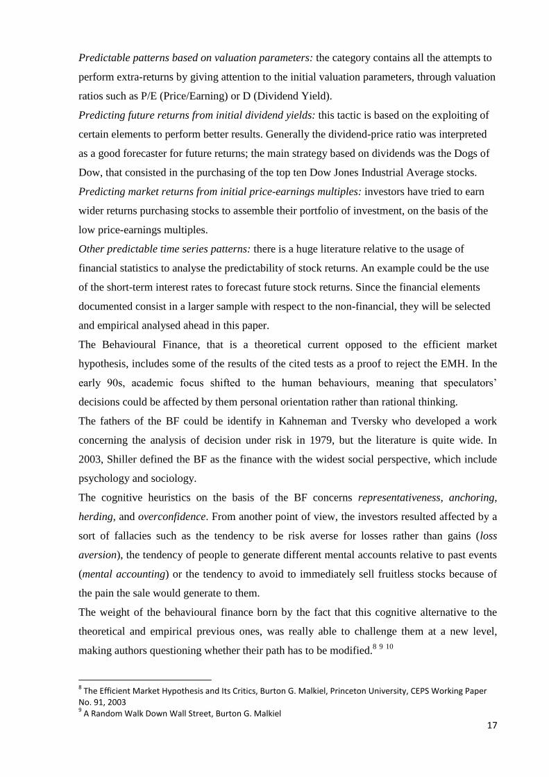
Predictable patterns based on valuation parameters: the category contains all the attempts to

perform extra-returns by giving attention to the initial valuation parameters, through valuation

ratios such as P/E (Price/Earning) or D (Dividend Yield).

Predicting future returns from initial dividend yields: this tactic is based on the exploiting of

certain elements to perform better results. Generally the dividend-price ratio was interpreted

as a good forecaster for future returns; the main strategy based on dividends was the Dogs of

Dow, that consisted in the purchasing of the top ten Dow Jones Industrial Average stocks.

Predicting market returns from initial price-earnings multiples: investors have tried to earn

wider returns purchasing stocks to assemble their portfolio of investment, on the basis of the

low price-earnings multiples.

Other predictable time series patterns: there is a huge literature relative to the usage of

financial statistics to analyse the predictability of stock returns. An example could be the use

of the short-term interest rates to forecast future stock returns. Since the financial elements

documented consist in a larger sample with respect to the non-financial, they will be selected

and empirical analysed ahead in this paper.

The Behavioural Finance, that is a theoretical current opposed to the efficient market

hypothesis, includes some of the results of the cited tests as a proof to reject the EMH. In the

early 90s, academic focus shifted to the human behaviours, meaning that speculators’

decisions could be affected by them personal orientation rather than rational thinking.

The fathers of the BF could be identify in Kahneman and Tversky who developed a work

concerning the analysis of decision under risk in 1979, but the literature is quite wide. In

2003, Shiller defined the BF as the finance with the widest social perspective, which include

psychology and sociology.

The cognitive heuristics on the basis of the BF concerns representativeness, anchoring,

herding, and overconfidence. From another point of view, the investors resulted affected by a

sort of fallacies such as the tendency to be risk averse for losses rather than gains (loss

aversion), the tendency of people to generate different mental accounts relative to past events

(mental accounting) or the tendency to avoid to immediately sell fruitless stocks because of

the pain the sale would generate to them.

The weight of the behavioural finance born by the fact that this cognitive alternative to the

theoretical and empirical previous ones, was really able to challenge them at a new level,

making authors questioning whether their path has to be modified.8 9 10

8 The Efficient Market Hypothesis and Its Critics, Burton G. Malkiel, Princeton University, CEPS Working Paper

No. 91, 2003 9 A Random Walk Down Wall Street, Burton G. Malkiel

18

2. Test on the EMH

2.1. An historical review

During the XX century a series of tests of the EMH have been implemented: the Dogs of the

Dow, the January effect, the Thank God it’s Monday afternoon pattern, the hot news

response, and so on. The Dogs of the Dow was a theoretical certainty that suggested how to

beat the market by means of the purchasing of the ten highest dividend yield stocks in Dow

Jones 30-Stock Industrial Average. This strategy was performed by Michael O’Higgins, while

tests on its truthfulness were effectuated by James O’Shaughnessy in 1920s. O’Shaughnessy

found out that this strategy really had been able to beat the index by over two percentage

points per year with no additional risk. This held as long as the strategy became too popular

and the market in turn beat the strategy.

Another reason that push researchers to do test on the efficiency of the market was the

unexplainable tendency of stock returns to be very high during the first two week of January.

Object of empirical examination was the week-end effect as well. The Thank God it’s Monday

afternoon pattern suggested that the best moment to purchase stocks was Monday afternoon

instead of Friday or Monday morning. This, because of the lower selling price with respect to

other moments.

The more intuitive doubt concerning the efficient market hypothesis is intuitively the

possibility that prices will immediately adjust for news when those come up. This doubt, for

instance, subsequent to the announcement of dividends, rather than earnings surprises, has

generated a literary trend called Event Studies.

At a later stage theories and tests which wanted to critically analyse the EMH branched out in

time series strategies and cross-sectional ones.

Time series strategies consist in the Dividend Jackpot Approach, the Trend is your friend one,

the Initial P/E predictor, and the Back we go again strategy. On the other hand, Cross-

sectional strategies include the Smaller is better effect.

The Trend is your friend is also known as the already cited Short-term momentum, while the

Dividend Jackpot Approach is based on the assumption that if stocks generate above-average

dividend yields, hence investors will earn higher future returns. This last approach was tested

first by Eugene Fama and Kennet French, and then, by John Campbell and Robert Shiller:

they concluded that, through this artifice, investors can reach their scopes. Obviously this

10

From Efficient Market Hypothesis to Behavioural Finance: Can Behavioural Finance be the new dominant model for investing?, A. Konstantinidis, A. Katarachia, G. Borovas, M. E. Voutsa, Scientific Bulletin – Economic Sciences, Vol. 11/Issue 2

19

was in contrast with the assumption of the randomness of the market. Tests showed that when

initial dividend yields were relatively high, investors would gain higher total rates of return.

Nevertheless, this eventuality does not seem to hold with an individual investor that simply

purchased a portfolio of individual stocks with the highest dividend yields and, in general,

does not seem to persist over time. Object of tests was the Back we go again strategy as well.

This strategy is better known as the Long-run return reversals and consisted in buying stocks

that did not perform very well in the latest years, convincing oneself that those stocks would

generate an above-average returns over the next few years. This depended on the fact that

tests underlined the possibility that, even if there existed positive correlation among stock

returns over short horizons, in term of years, they showed negative serial correlation. This

would lead to gain extra-returns. In his revisionary work A Random Walk Down Street,

Malkiel accepted the truthfulness of this latest strategy mentioned, asserting that fads and

fashions can play a central role in stock pricing.

Moving on in the historical review of the tests over the EMH and its anomalies, the Smaller is

better effect comes up. It starts from the fact that small company stocks generate larger

returns than large company stocks do.11

Fama and French divided stocks into deciles according to their size finding out that small

firms outperformed larger ones. On the other hand, this could be not true, because it has to be

considered that small firms provide higher risks to investors.

Finally there have to be hinted the Stocks with low price-earnings multiples outperform those

with high multiples approach, also described as the GARP approach, that was tested by

Sanjoy Basu during the 70, besides another pattern relatively recently tested, considering the

relation between the ratio of stock’s price to its book value and its later return, the P/BV

(Price-to-book-value).

In general, the approach for the EMH consisted in statistical tests in security prices and

returns or tests based on trading rules. Obviously, trading rules are not disclosed as much as

tests because if someone found out a good strategy, he/she would not explain it to his/her

trading competitors. Therefore the focus is put on econometrical tests.

For what concerns the weak-form of the efficient market hypothesis, some examples of tests

are:

- Autocorrelation (serial correlation) tests

- Runs tests

- Sings tests

- Unit root tests 11

A Random Walk Down Wall Street, Burton G. Malkiel

20

Semi-strong-form of the EMH have been tested in three different ways:

- Through the usage of time series analysis over public information (Dividend yield; Default

Spread; Term structure spread; Quarterly earnings reports information)

- Through the examinations raised up by Event Studies (the object of these studies is the stock

response time to economic events)

- Through cross-sectional analysis of returns over public information. This trend bases its

efforts on the assumption that in an efficient market securities have risk-adjusted returns (P/E

ratios; Price-Earnings/Growth ratios; The size effect; Book value-Market value)

Among the Autocorrelation Tests, used in order to verify the presence of dependence in data

series, so used to verify whether each value of the time series considered is influenced by the

previous value and, in the same way, influences the following one, it is possible to find the

following ones:

Durbin-Watson Test: this is the first attempt to test for serial correlation in a linear time series

model as:

𝑦𝑡 = 𝑥𝑡𝑇𝛽 + 휀𝑡 𝑤𝑖𝑡ℎ 휀𝑡~𝑊𝑁(0, 𝜎2) (17)

It consists is a statistic (rather than a test) that helps to find out whether residual serial

correlation exists or not.

The DW-Statistic is based on the following structure:

{𝐻0: 𝑃1 = 0 𝑛𝑜 𝑓𝑖𝑟𝑠𝑡 𝑜𝑟𝑑𝑒𝑟 𝑠𝑒𝑟𝑖𝑎𝑙 𝑐𝑜𝑟𝑟𝑒𝑙𝑎𝑡𝑖𝑜𝑛

𝐻0: 𝑃2 ≠ 0 𝑓𝑖𝑟𝑠𝑡 𝑜𝑟𝑑𝑒𝑟 𝑠𝑒𝑟𝑖𝑎𝑙 𝑐𝑜𝑟𝑟𝑒𝑙𝑎𝑡𝑖𝑜𝑛

Here is the formula:

𝐷𝑊 =∑ (�̂�𝑡−�̂�𝑡−1)2𝑇

𝑡=2

∑ 𝜀𝑡2𝑇

𝑡=1 (18)

With 휀�̂� corresponding to the OLS residual.12

Breusch-Godfrey Test: this is a test that allows statisticians to understand whether exists or

not serial dependency in the variation of the dependent variable (in a dynamic linear model).

It differs from the DW-statistic because of the possibility to test different serial correlation

orders. The structure of the hypothesis is the following:

12

Dispensa di Econometria delle Serie Storiche, Giulio Palomba, 2014 (P.10)

21

{𝐻0: 𝜌1 = 𝜌2 = 𝜌3 = ⋯ = 𝜌𝑞 = 0

𝑡ℎ𝑒𝑟𝑒 𝑒𝑥𝑖𝑠𝑡𝑠 𝑎 𝜌𝑖 ≠ 0, 𝑤𝑖𝑡ℎ 𝑖 = 1,2,3, … , 𝑞

It is a test based on Lagrange multipliers that is approximated as follow:

𝐿𝑀𝐵𝐺 = 𝑇𝑅2~𝑥𝑞2 (19)

Where 𝑅2 is the auxiliary regression and T the largeness of the sample case.13

Ljung-Box Test: this is a test to establish if observations over a given time series are serial

correlated. The null hypothesis foresee the absence of serial correlation:

{𝐻0: 𝜌1 = 𝜌2 = 𝜌3 = ⋯ = 𝜌𝑞 = 0

𝑡ℎ𝑒𝑟𝑒 𝑒𝑥𝑖𝑠𝑡𝑠 𝑎 𝜌𝑖 ≠ 0, 𝑤𝑖𝑡ℎ 𝑖 = 1,2,3, … , 𝑞

So, the LB-statistic is:

𝐿𝐵 = 𝑇(𝑇 + 2) ∑𝜌�̂�

𝑇−𝑖~𝑋𝑞

2𝑞𝑖=1 (20)

The Runs Tests could be a mean to understand if a data sample follows a random process.

The runs test hypothesis follows the trend below:

{𝐻0: 𝑡ℎ𝑒 𝑠𝑒𝑞𝑢𝑒𝑛𝑐𝑒 𝑖𝑠 𝑟𝑎𝑛𝑑𝑜𝑚

𝐻1: 𝑡ℎ𝑒 𝑠𝑒𝑞𝑢𝑒𝑛𝑐𝑒 𝑖𝑠 𝑛𝑜𝑛 − 𝑟𝑎𝑛𝑑𝑜𝑚

The statistic of the Runs test is the following:

𝑍 =𝑅−𝑅

𝑠𝑅 (21)

Where R is the observed number or runs and 𝑅 is the expected number of runs. s is the

standard deviation.

The Sing Test is a non-parametric test to verify the central tendency. In other words, a sign

test tries to verify the central value for a probability distribution.

The null hypothesis is represented hereinafter:

13

Dispensa di Econometria delle Serie Storiche, Giulio Palomba, 2014 (P.12)

22

{𝐻0: 𝜇 = 𝜇0

𝐻1: 𝜇 ≠ 𝜇0

It uses the median. In order to perform bilateral tests, the sign test verifies the following

hypothesis:

{𝐻0: 𝑚𝑒 = 𝑚𝑒0

𝐻1: 𝑚𝑒 ≠ 𝑚𝑒0

In the case of unilateral test the hypothesis are:

{𝐻0: 𝑚𝑒 ≤ 𝑚𝑒0 𝑣𝑠 𝐻1: 𝑚𝑒 > 𝑚𝑒0

𝑜𝑟𝐻0: 𝑚𝑒 ≥ 𝑚𝑒0 𝑣𝑠 𝐻1: 𝑚𝑒 > 𝑚𝑒0

The sign test is the non-parametric equivalent of the t test, but it differs because of the

binomial distribution. In the practice, each value of the sample is compared with a defined

value in order to transform lower values in negative signs and higher values in positive ones.

The null hypothesis is not rejected when positive and negative signs appear approximately

equal.14

15

Economic and financial series are characterized by the property of non-stationarity, as a

consequence statisticians tends to transform them by means of differentiation, logarithms, or

logarithmic differences. It is necessary to verify if the time series under analysis are

integrated, hence Unit Root Tests come to help testers.

Unit root tests try to verify the presence of a stochastic trend in a series. It consists of two

different tests. Tests diverge for the null hypothesis. The first one follows the system below:

{𝐻0: ∅ = 1

𝐻1: |∅| < 1

The null hypothesis states that the generator process of 𝑥𝑡 is I(1), integrated of order one,

while the alternative is represented by an autoregressive stationary process.

While the second test follows this other system:

14

Introduzione alla statistica non parametrica, Luigi Salmaso 15

Elementi di Statistica Descrittiva per distribuzioni univariate, Metodi non parametrici per un campione, Maria Pia D’Ambrosio, Franco Anzani, Six Sigma

23

{𝐻0: |∅| < 1𝐻1: ∅ = 1

Therefore, in the second test, the null hypothesis is given by the absence of the non-stationary

process, that is, on the other hand, present in the alternative hypothesis.16

17

Here we have the main tests normally used:

Augmented Dickey-Fuller Test (ADF): it is an univariate test. It uses an autoregressive

parametric model. The ADF test is based on estimating the following regression:

𝑦𝑡 = 𝛽𝑇𝐷𝑡 + 𝜑𝑦𝑡−1 + ∑ 𝜓𝑗∆𝑦𝑡−𝑗 + 휀𝑡𝑝𝑗=1 (22)

Where:

- 𝐷𝑡 is a vector of deterministic terms (constant, trend etc.).

- The p-lagged difference terms, ∆𝑦𝑡−𝑗 are used to approximate the ARMA structure

of the errors.

- p is set so that the error ε t is serially uncorrelated. T휀𝑡homoskedastic.

Phillips-Perron Test: it is used to test the null hypothesis over unit roots. It is based on the

following regression:

𝑦𝑡 = 𝛽𝑇𝐷𝑡 + 𝜑𝑦𝑡−1 + 𝑢𝑡 (23)

Where:

- 𝑢𝑡 is an I(0) process that can be heteroskedastic. This is the main difference between the ADF

and PP test.

On the other hand, talking of semi-strong tests, it is opportune to introduce the concept of

Event Study. This discipline has the aim to understand the impact of a specific event over a

firm’s value by means of financial data. Otherwise, event studies study whether a certain

event would change or not the course of stocks. At a later stage the semi-strong test branch

would be deeper examined.

16

Dispensa di Econometria delle Serie Storiche, Giulio Palomba, 2014 17

Introduzione all’econometria, N.Cappuccio, R.Orsi

24

2.2. Previous studies: the Italian cases

In Italy there were different authors focusing on the efficient market hypothesis question.

Among them, Franco Caparrelli could be intended as the main exponent.

He performed several tests on the Italian market18

19

20

21

, considering the whole market

efficiency concept. He tested for weak, semi-strong and strong form. Let’s see in the next step

how he proceeded in his analysis.

2.2.1 The Weak-form

This first form elaborated under the EMH, states that the knowledge given by the past does

not allow investors to have a better performance over stocks.

It is possible to sum up this hypothesis as follow:

𝑍𝑡−1 = 𝑍𝑡−1∗ 𝐸(𝑅𝑡/𝑍𝑡−1) = 𝐸(𝑅𝑡/𝑍𝑡−1

∗ ) (24)

Where 𝑍𝑡−1 corresponds to the prices, returns and exchanged volumes time series.

This form considers information as free and available for investors with homogeneous

expectations in a transaction-costless market. This would lead to two consequences: there

exist no mispriced stocks and there exist no possibility that an investor could follow an

established path to earn extra-profit.

So, the first study Capparelli performed was about 30 securities during the period from

December 1978 to December 198322

.

In his book, Il Mercato Azionario, Caparelli synthetized results of the serial correlation test

as follow:

Daily Weekly Fortnightly Monthly

�̅� -0.1268 -0.1167 0.0139 0.0403

𝜎 0.1885 0.1394 0.1529 0.1172

𝜎/𝜎(𝛽) 2.9921 2.2520 1.7434 0.9002

Terms number

> 2𝜎(𝛽) 15/30 11/30 4/30 1/30

18

La reazione in eccesso del prezzo dei titoli: la teoria e una verifica empirica sulle azioni italiane, Franco Caparrelli e Anna Maria D'Arcangelis, Bancaria, 51(10), 1995, pp. 8-17 19

Mercato efficiente ed effetto gennaio, Franco Caparrelli et al., Il Risparmio, (1), 1992, pp. 33 20

Quando comprare e vendere in Borsa. Una verifica dell'effetto fine settimana, Franco Caparrelli e Alessandra Diotallevi, Bancaria, (5), 1991, pp. 27 21

La Borsa italiana e l'efficienza semiforte, Il Risparmio, (2), 1989, pp. 209 22

Il Mercato Azionario, Franco Caparelli

25

Positive terms

number 8/30 7/30 13/30 19/30

Table 2.1 – Summary of results for the correlation test 12/1978-12/1983, F. Caparrelli

Where �̅� represents the mean value of the coefficient 𝛽, 𝜎 is the standard deviation, and > 2𝜎(𝑟)

represents the number of terms higher than 2𝜎(𝑟).

This table shows that the hypothesis holds better if monthly data are considered instead of the

weekly ones. Indeed the mean value of 𝛽 reduces. The number of the securities with a

coefficient equals to zero decrease as well. Therefore the more the time interval grows the

more the empirical result resembles the theory (meaning that the true value of the coefficient

is equal to zero).

2.2.1 The Semi-strong-form

This form states that public information are quite instantaneous transferred into stock prices,

as a consequence the knowledge of those information cannot produces the possibility to get an

advantage over the market.

These information come from the study of companies through their balance sheets, the

announcements of results, as well as programs and perspective of the companies themselves.

Caparrelli examined 54 events of free share capital increase (intend aumenti di capitale a

titolo gratuito – questa dovrebbe essere una traduzione migliore) from January 1975 to April

1987 relative to securities quoted on the stock exchange of Milan. This study focused the

attention on the period before and after the announcement of dividends. The first phase was to

define the market model for each stock over 148 months, and so defining alpha and beta

coefficients. Then Caparrelli found out the expected returns with the aim to compare them to

the effective ones. Finally he calculated the simple average residual and the cumulated one.

This analysis underlined that there was an increment of stocks and profits since the moment of

the announcement, but this increment had been balanced out in two months.

Another experiment was performed considering the period from October 1990 to August

1993. This test was based on the suggestion given by the column “Quanto valgono – Otto

azioni ai raggi X degli esperti” of the magazine “Milano Finanza”. The sample was composed

of 231 purchasing suggestions against 67 selling suggestions. This study utilized the

technique of the event study through the statistic suggest by Brown and Warner:

∑ 𝑒𝑡 / ∑ 𝜎[𝑒𝑡(𝑚)] (25)

26

The mentioned statistic consists in the ratio between the average residual of the day t and the

estimation of the standard deviation of the average residuals during the period before the

beginning of the test.

Hereunder the results of the test with the daily average residuals:

Average Residual

Days Purchases t-Stud Sales t-Stud

-10 -0.151 -0.804 0.097 0.272

-9 -0.107 -0.568 -0.174 -0.489

-8 0.040 0.212 -0.248 -0.697

-7 -0.222 -1.181 0.136 0.383

-6 0.127 0.677 -0.066 -0.185

-5 -0.113 -0.601 0.212 0.597

-4 0.193 1.029 -0.574 -1.614

-3 0.379 2.017 -0.405 -1.141

-2 0.035 0.185 -0.436 -1.228

-1 0.168 0.896 0.076 0.215

1 0.542 2.883 -1.021 -2.873

2 0.268 1.425 -0.299 -0.841

3 0.024 0.127 -0.332 -0.933

4 -0.156 -0.828 -0.621 -1.749

5 -0.252 -1.339 0.327 0.921

6 0.164 0.873 -0.257 -0.723

7 0.175 0.931 -0.595 -1.674

8 -0.114 -0.607 0.458 1.290

9 -0.039 -0.209 0.318 0.895

10 0.095 0.506 -0.364 -1.023

Table 2.2 – Summary of results 10/1990-8/1993, F. Caparrelli

Results did not permit to refuse the null hypothesis that residuals are not correlated.

2.2.2 A continuing process

Tests to confirm or refuse the EMH have been carried on for years even now some authors try

to perform new ones.

Indeed very recently, another form to test the semi-strong hypothesis has been developed. On

February 26, of the current year, Arianna Ziliotto and Massimiliano Serati of the Carlo

27

Cattaneo LIUC University School of Economics and Management, published The Semi-

Strong Efficiency Debate: in Search of a New Testing Framework. They built their idea on the

basis that focusing just on return distribution and profit opportunities would twist the mean of

the tests.

Their model is based on a Testing Tree that consists of three steps:

Step 1: Market Surprise

Step 2: Volatility

Step 3: Spillovers

Figure 2.1 Testing Tree, The Semi-Strong Efficiency Debate: in Search of a New Testing Framework

In the first step it is possible to understand whether there exist market surprise, and so there is

no anticipation of any information, or whether there exist no market surprise, and so there is

the need to investigate. The second step lead to another investigation choice with respect to

the degree of the volatility, evidencing the need to further investigation patterns in presence of

low volatility of the market. Finally the model focuses on spillover effects, exploiting their

impact on the market to discriminate on the existence of the efficiency.23

23

The Semi-Strong Efficiency Debate: in Search of a New Testing Framework, Arianna Ziliotto, Massimiliano Serati, Carlo Cattaneo LIUC University School of Economics and Management, February 2015

28

3. Anomalies on the EMH

As it has been showed hereby, the efficient market hypothesis consists of three forms.

However, the most practical and interesting form is the semi-strong efficiency form. During

the literature evolution researchers have found interesting way to test this form because of the

evidence coming from the market. Dividends announcements, multiple ratios based on price

and earnings, calendar events, etc.. are elements came to light by the investigation over the

semi-strong form. This branch is known as Anomalies of the Efficient Market Hypothesis. In

other words, the anomalies indicate inefficiency into markets, or rather a situation in which

stocks deviate from the assumption of the EMH. Often this inefficiency has been proved not

to be persistent once discovered, despite this interpretation is not always true. Indeed, after the

documentation of an anomaly, there exist three possibility: the anomaly will disappear,

reverse or attenuate. This leads to some question regarding the possibility to forecast these

anomalies in order to get advantage over the market. On the other hand an anomaly could be

the proof of the inadequacy of the model undertaken.

The anomalies branch has developed its literature since 80s as a consequence of the attention

previously conferred to the efficient market investigation. Here, the purpose of researchers

was to find out some systematic variations of the stock price. This working field is quite

interesting because it allows to compare different markets, and so, it allows to understand

whether markets follow the same rules. At the end of 80s Samuelson stated that finance was

not anymore a perfect model, but it would be possible to accept the presence of anomalies into

markets. This was the first step for opening the doctrine doors to events that the current

doctrine could not explain.

According to Latif et al. (2011) it is possible to distribute anomalies into three basic area:

Fundamental anomalies, technical anomalies and calendar (or seasonal) anomalies. Most

common anomalies concerned rates of change on the basis of variations in specific temporal

circumstance.24

3.1 Calendar Anomalies

This category consists of those effects, based on the calendar, which are cyclical in returns.

Most of the calendar effects have been diminished, disappeared or reversed as affirmed above.

Calendar anomalies are observed in presence of each significant change in time: year, month,

24

Market Efficiency, Market Anomalies, Causes, Evidences, and Some Behavioral Aspects of Market Anomalies, M. Latif, S. Arshad, M. Fatima, S. Farooq, Institute of Management Sciences Bahauddin Zakaria University, Multan, Pakistan, 2011

29

week or day. They became popular because of their huge typology and their affordable

investigation. Calendar anomalies still face controversial opinion over their existence,

especially by whom support the idea that transaction price would cancel them. In any case, it

is possible to list the most common anomalies:

Week-end/Monday effect

January effect

Holidays effect

Intraday effect

Halloween effect

Turn of the month effect

3.2 The week-end effect

In 1973 F. Cross observed for the period 1953-1970 that the Stock Exchange Index has highly

positive changes on Friday with respect to the other days, otherwise there were less

increments on Monday. In 1980 Kenneth French disclosed an anomaly that consisted in the

production of negative average return over weekends. French studied the Standard and Poor’s

(S&P) portfolio in the period 1953-1977. This analysis was integrated by Schwert including

estimations of the weekend effect from February 1885 to May 2002, and other sample periods

not included in French’s study. The starting point was the following regression:

𝑅𝑡 =∝0+∝𝑤 𝑊𝑒𝑒𝑘𝑒𝑛𝑑𝑡 + 휀𝑡 (26)

Where Weekend = 1 when the return spans Sunday, and zero otherwise. ∝𝑤 represents the

difference in average return over the weekend versus other days. 25

Hereinafter the results of the estimation:

Sample period 𝛼0 𝑡(𝛼0 = 0) 𝛼𝑤 𝑡(𝛼𝑤 = 0)

1885-2002 0.0005 8052 -0.0017 -10.13

1885-1927 0.0004 4.46 -0.0013 -4.96

1928-1952 0.0007 3.64 -0.0030 -6.45

1953-1977 0.0007 6.80 -0.0023 -8.86

1978-2002 0.0005 4.00 -0.0005 -1.37

Table 3.1 Day-of-the-week effects in the U.S. stock returns, Anomalies and Market Efficiency. G. William

Schwert

25

Anomalies and Market Efficiency. G. William Schwert, University of Rochster, and NBER, 2003

30

The coefficient aw appears negative when the returns over the weekend are lower than the

ones in the other days. From data is evident that results from test have become less negative,

underlying that the effect studied have started decreasing (or at least attenuating ) since 80s

(the discovered of the weekend effect). It leads to understand that the variance per time unit of

the differences in price series is slower in the weekend. This means that Monday’s price is the

result of a random walk process that lasts three days. Following this ideology and starting

again from daily data (1975-1989, historic MIB index by Milan Stock Exchange), Barone

tried to verify whether the velocity of the stock prices generating process would change when

markets are supposed to be closed. Therefore, in 1990, he published his study where standard

deviations and averages of the index MIB rates were divided day by day. The rate averages

resulted negative on Monday and Tuesday, and positive on Friday. Even the stock generating

process velocity (standard deviation) resulted higher on Monday.26

Moreover Barone tested the same sample also by means of a regression:

𝑅𝑡 = 𝑎1 + 𝑏2𝐷2 + 𝑏3𝐷3 + 𝑏4𝐷4 + 𝑏5𝐷5 + 𝑢𝑡 (27)

Where 𝐷2 is a dummy for Tuesday (𝐷2 = 1 if the observation falls on Tuesday, 𝐷2 = 0

otherwise), 𝐷3 is a dummy for Wednesday, and so on as follow:

𝐷2 =1 𝑖𝑓 𝑡ℎ𝑒 𝑟𝑒𝑡𝑢𝑟𝑛 𝑏𝑒𝑙𝑜𝑛𝑔𝑠 𝑡𝑜 𝑇𝑢𝑒𝑠𝑑𝑎𝑦

0 𝑖𝑓 𝑡ℎ𝑒 𝑟𝑒𝑡𝑢𝑟𝑛 𝑏𝑒𝑙𝑜𝑛𝑔𝑠 𝑡𝑜 𝑡ℎ𝑒 𝑜𝑡ℎ𝑒𝑟 𝑑𝑎𝑦𝑠

𝐷3 =1 𝑖𝑓 𝑡ℎ𝑒 𝑟𝑒𝑡𝑢𝑟𝑛 𝑏𝑒𝑙𝑜𝑛𝑔𝑠 𝑡𝑜 𝑊𝑒𝑑𝑛𝑒𝑠𝑑𝑎𝑦

0 𝑖𝑓 𝑡ℎ𝑒 𝑟𝑒𝑡𝑢𝑟𝑛 𝑏𝑒𝑙𝑜𝑛𝑔𝑠 𝑡𝑜 𝑡ℎ𝑒 𝑜𝑡ℎ𝑒𝑟 𝑑𝑎𝑦𝑠

𝐷4 =1 𝑖𝑓 𝑡ℎ𝑒 𝑟𝑒𝑡𝑢𝑟𝑛 𝑏𝑒𝑙𝑜𝑛𝑔𝑠 𝑡𝑜 𝑇ℎ𝑢𝑟𝑠𝑑𝑎𝑦

0 𝑖𝑓 𝑡ℎ𝑒 𝑟𝑒𝑡𝑢𝑟𝑛 𝑏𝑒𝑙𝑜𝑛𝑔𝑠 𝑡𝑜 𝑡ℎ𝑒 𝑜𝑡ℎ𝑒𝑟 𝑑𝑎𝑦𝑠

𝐷5 =1 𝑖𝑓 𝑡ℎ𝑒 𝑟𝑒𝑡𝑢𝑟𝑛 𝑏𝑒𝑙𝑜𝑛𝑔𝑠 𝑡𝑜 𝐹𝑟𝑖𝑑𝑎𝑦

0 𝑖𝑓 𝑡ℎ𝑒 𝑟𝑒𝑡𝑢𝑟𝑛 𝑏𝑒𝑙𝑜𝑛𝑔𝑠 𝑡𝑜 𝑡ℎ𝑒 𝑜𝑡ℎ𝑒𝑟 𝑑𝑎𝑦𝑠

𝑎1 is the average rate of change on Monday, while 𝑏𝑛 represents the difference of the average

rate of change on the other days.

26

Aspects of Market Anomalies, M. Latif, S. Arshad, M. Fatima, S. Farooq, Institute of Management Sciences Bahauddin Zakaria University, Multan, Pakistan, 2011

31

Period Degree of freedom Ordinary Least Squares Generalized Least squares

F Confidence

level

F Confidence

level

1975-1989 4 3384 6,69 0,000 6,95 0,000

1975-1979 4 1129 3,02 0,017 2,88 0,022

1980-1984 4 1169 2,37 0,050 2,50 0,041

1985-1989 4 1076 3,16 0,013 3,18 0,013

Table 3.2 Il Mercato Azionario Italiano: efficienza e anomalie di calendario, E. Barone, 1990

The zero-hypothesis (𝐻0: 𝑏2 = 𝑏3 = 𝑏4 = 𝑏5 = 0) has been tested in the chart above. Results

show that it is possible to reject the hypothesis at a confidence level of 95%. Rates of change

on Monday appears reliably different from the others.

It is important to mention that the test used in this context was the F statistic of Snedecor:

𝐹 =[

𝑅2

(𝑘−1)]

[(1−𝑅2)

(𝑛−𝑘)] (28)

With k and n-k degrees of freedom, where k represents the number of independent

(forecasting) variables and n the number of observations:

It is possible to note that Barone did not report just the OLS data, but the GLS too. He found

out that standard deviations results could suffer an heteroskedastic problem and so it would be

better to standardize variables in the regression (27). As reported, he included in the analysis

the generalized least squares contribution, underlying how results did not change. 27

So, this test underlined how the rates of change on Monday were reliably different from the

ones on the other days of the week.

M. Gibbons and Hess got results quite similar to French using a linear regression model with

different dummies. Indeed these dummies represented the expected returns of the various days

instead of the difference with respect to Monday.

3.2.1 Other calendar anomalies

As aforementioned, there exist some other anomalies. An interesting anomaly is the holiday

effect: Jacobs and Levy noted that the 35 percent of stocks growth in 1963-1982 occurred in

the eight non-working days of the year. This leads to understand that this effect often occurs

27

Il Mercato Azionario Italiano: efficienza e anomalie di calendario, E. Barone, 1990

32

on the national days, in the new year’s day, etc. It is possible to distinguish between pre-

holiday effect and post-holiday effect, both representing a change of direction in stock prices

flow. Therefore, the holiday effect consists in a better performance on days preceding a

holiday, and in a worst performance on next days. In 1990 Ariel verified a significant

increment of stocks returns before Christmas and before the May Day with respect to other

holidays.

Recently, Tamara Backovic Vulic tested this effect over the 13th

July (Montenegrin Statehood

day) for the period 2003-2009. Some results could be appreciated in the following graphic:

Figure 3.1 Testing the Efficient Market Hypothesis and its Critics - Application on the

Montenegrin Stock Exchange, Tamara Backovic Vulic,

These results showed that this effect is not really effective in Montenegro, apart from two

deducible cases.28

The January effect has been the main famous calendar anomaly. It consists in a reliably higher

rate of changes for every stocks in the month of January (with respect to the other months).

For what concerns the Italian market, Giannasca and Macchiati (1986) discovered a strong

seasonality in 1975-1989. Results based on the historic MIB showed rates of change equal on

average to 0.33 per cent and significantly different from zero at a confidence level of 0.001

per cent. It is possible to observe these results in the following figure.

28

Testing the Efficient Market Hypothesis and its Critics – Application on the Montenegrin Stock Exchange, Tamara Backovic Vulic, MSc University of Montenegro, Podgorica Faculty of Economics, professor assistant of Econometrics, Business Statistics, Operations Research, Applied Econometrics and Decision Making Models

33

Figure 3.2 Il Mercato Azionario Italiano: efficienza e anomalie di calendario, E. Barone, 1990

As stated by Caparelli, there are evidences of the prevalence of the January effect over the

weekend effect. In fact the average return on Monday and Tuesday is resulted positive in

January although it resulted negative during the other months:

Average

Return

Monday Tuesday Wednesday Thursday Friday

January -0.26% 0.23% 0.27% 0.25% 0.40%

Other months -0.08% -0.17% 0.14% 0.10% 0.15%

Table 3.3 Il Mercato Azionario, F. Caparrelli

Rozeff and Kinney verified the presence of the January effect on a sample of stocks by the

New York Stock Exchange in 1904-1974, observing higher returns concentrated in the first

fifteen days of the month. The January effect has been justified by psychological belief that

investors are affected by the conviction that the new year could start positively, or rather, as

affirmed by Jacob and Levy, that investors usually wait the new year to sketch out a new

strategy on the basis of the expected scenario proposed by analysts.

It is appropriate to hint the turn-of-the-month effect. The mere turn of the month seemed to be

able to lead investors buying securities. This is confirmed by the fact that the rates of change

at the beginning and at the last five days of the month appeared to be deeply positive pursuant

to Ariel’s work (1987). On the other hand, on the basis of Caparelli’s work, the Italian market

34

appeared to show stock prices lower in the first part of the month (when the trading cycle ends

up) and higher in the second part. However it is evident that these results could be affected by

other anomalies such as the afore-mentioned January effect.

Boido et al. (2004) observed the summer-time (or daylight savings time) effect by means of

the COMIT index. Results showed the presence of the effect on the basis of the fact that the

time after the change of hour underlined a different prices average. In addition, days next to

the daylight savings time moment appeared to get an average index value higher than the

general mean. 29

3.3 Fundamental Anomalies

It is possible to gather together some anomalies under the name of fundamental anomalies by

underlying the ones that appear to have some value for individual investors on the basis of

financial reports. This section includes P/E effect, Book-to-Market ratios, Earnings

announcements, Neglected-firm effect, High Dividend effect, and so on.

Going deeper in each meaning it is possible to briefly define these anomalies. The dividend

yield anomaly states that high dividend yield stock outperforms the market with respect to the

lower ones. Price to earnings ratio anomaly supported the idea that portfolio composed of low

P/E stocks often outperform portfolios composed of high P/E stocks. In the same way stocks

of companies with high book-to-market ratios outperform stocks with low book-to-market

ratios. Moreover this effect seems not to be dependent on systematic risk, but on the fact that

companies with low book-to-market ratios are perceived to be companies that grow rapidly.

Earnings announcements can have variable effects on stock prices, their effects basically

depend on analysts interpretation of the market in pursuit of predictability through earnings

expectations published on website or personal relationships with experts. Again,

the neglected-firm effect occurs on stocks that has lower trading volume in addition to the

approximately absence of analysts support. It is possible to going on listing these anomalies,

but a more advisable way is to examine one of them deeper.30

3.4 The P/E effect

It has been stated that this effect asserts that the stock with low price to earnings ratio are

likely to generate higher returns outperforming the market, while the stocks with high price to

29

Anomalie di calendario: l'effetto ora legale, Boido, Claudio, Fasano, Antonio, Periodico: AF. Analisi finanziaria, 2004 30

The neglected firm effect and an application in Istanbul Stock Exchange, Soner Akkoc, Mustafa Mesut Kayali, Metin Ulukoy, Banks and Bank Systems, Volume 4, Issue 3, 2009

35

earnings ratios tend to underperform with respect to the same market. The P/E ratio is

calculated as the following ratio:

𝑃

𝐸=

𝑃0

𝐸𝑃𝑆 (29)

Where 𝑃0 is the price of the security at time zero, and EPS is the earning per share calculated

as the ratio between the last reported earnings and the number of stocks.

Among the various hypothesis over the meaning of the P/E effect, there exist some based on

the CAPM and others based on risks attitude. Following this concept, low P/E stocks are

assumed to be risker than high ones (this means that the β of the low P/E stocks is greater than

the β of the high P/E ones), and therefore they would generate higher performance.

Nevertheless further studies demonstrated that the leakage between low P/E and high β was

not enough to explain the anomaly. Portfolio considered appeared to show greater

performances even after the analysis started including risk. In 1977 Basu performed a study

on this effect. His analysis followed this outline:

Calculation of the P/E ratio for each security of the sample

Composition of five portfolios on the basis of the P/E value

Calculation of the monthly return for each portfolio

Re-composition of portfolio (after 12 months)

β coefficient estimation for each portfolio and indexes estimations

Results showed that the greater performance of low P/E samples was not related to an higher

value of the systemic risk.

In 1994 Calcagnini and D’Arcangelis examined a sample of 42 securities for the period 1979-

1992. They constructed some portfolios on the basis of the P/E ratio supposing to buy them at

the beginning of the year and hold them for the whole year. Then it was constructed the

market model to evaluate the performance on the basis of the systemic risk. Results showed

unsatisfactory conclusions: in the long run the connection between low P/E and high

performance seemed to hold, but there were no possibility to reject the equality hypothesis on

the basis of the significance test of portfolio return differences.

Returns and statistics Portfolios

1 2 3

Average P/E 8.27 17.18 57.71

Average return of the year 48.22 40.12 32.86

36

Systemic Risk (β) 1.03 0.99 0.92

Return/β 46.77 40.42 35.75

Table 3.4 Il Mercato Azionario, F. Caparrelli

3.4.1 Other fundamental anomalies

Akkok et al. (2009) studied the neglected-firm effect in 1999-2008 (Istanbul Stock Exchange)

using monthly volume data. They found out that the portfolio they have constructed by

popular stocks earned the highest abnormal return when compared to the abnormal returns

earned by the other two portfolios constructed consisting of neglected and normal stocks. This

leads to understand that ISE (Istanbul Stock Exchage) was not affected by the neglected-firm

effect, even if previous tests have documented some evidences. Popular stocks showed higher

average with respect to the portfolio consisting of neglected stocks in all years but 2008.

Furthermore the monthly average abnormal return of neglected portfolio is negative.

Moreover t-test showed values for popular portfolio which were statistically significant in

each year, t-values for normal portfolio were statistically significant in 7 years out of 10 years

and the ones for neglected portfolio were significant in all years but 2008 at the 5% level.

They tried to establish whether their results were a consequence of the January effect as well.

However they got same results and concluded their findings were not consistent with the

January effect, contradicting the Neglected-firm effect.

Brian T. Brian T. Allman et al. gave a contribute to the Small-firm effect research analysing

NYSE and AMEX stock prices in 1962-1975. They found out that portfolios of smallest firm

on average experienced returns over 20% which were reliably higher than portfolios of largest

firms. There were evidences that allow to think that investors could construct portfolios with

systematically abnormal returns on the basis of firm size31

.

3.5. Technical Anomalies

For technical anomalies it has been considered the techniques used to forecast future prices of

stocks on the basis of past prices and past information which seemed to have some effect on

markets. So, the purpose of the technical analysis is to study time series and exchanged

volumes without considering the object, this raised some interesting anomalies. Among the

anomalies identified in the technical field we found the Moving Averages and the Trading

Range beak.

3.5.1 Hints on technical anomalies

31

The Size Effect, Brian T. Brian T. Allman et al, 2009

37

Hons and Tonks examined trading strategies in the US Stock Market founding signs of

momentum strategies during the period 1977-1996. They discovered the possibility to gain

advantages by past positives securities. Hence, the momentum anomaly states that securities

that reliably went up in the past would probably continue to go up in the near future. This

means that stocks which outperform on the short run period tend to perform well also in the

future. The momentum strategy is based on the assumption that price of securities are more

likely to keep moving in the same direction, than to change it. Momentum effect has been

proved to be effective in the US Small and Large Cap universe32

. Resistance and support level

are the basis of the Trading Range Break strategy. Support level represents the level of price

corresponding a break in the negative trend of a stock, while resistance level represents an

abstract level in which prices stops to grow. Support level occurs when a big amount of

purchasing affect those stocks which have performed negative trends, while resistance occurs

when many stock sales take place at the same time. A trading range break tries to forecast

and exploit these circumstances. A price penetrating the resistance level would generate a buy

signal while a price penetrating the support level would generate a sell signal. The belief is

that investors sell at the resistance level and buy at the support level. In 1992 Brock et al.,

analysed the above-mentioned effect on the Dow Jones Industrial Index from 1897 to 1985.

They found out that this technical analysis would be effective against the market unless costs

should be not carefully took into account since the beginning. Obviously there are contrasting

examination on technical anomalies, but they are not be examined here.

3.6. Do famous anomalies persist nowadays?

This is a conflicting issue. The persistence of the anomalies appeared over the time do not

persuade everyone. In 2002 Schwert observed that all the well-known anomalies in the

finance literature do not hold up in different sample periods. Examples could be represented

by the size and the value effects, which seem to have disappeared after the papers their

existence have been brought to light.

In certain market happen that even the weekend and the dividend yield effect decreased their

predictive power.

The small-firm turn-of-the-year effect became weaker in the years after it was first

documented in the academic literature, although there is some evidence that it still exists.

32

Does Momentum Investing Work?, Alex Bryan, 2013 (http://ibd.morningstar.com/article/article.asp?id=591675&CN=brf295,http://ibd.morningstar.com/archive/archive.asp?inputs=days=14;frmtId=12,%20brf295)

38

The reason might be the popularity these anomalies achieve. In other words, investors that

have been able to experience these anomalies, have tried to exploit them to beat the market as

well. Moreover once anomalies have been discovered, prices could be corrected by operators

on the basis of new information received.

Hence, Schwert suggested that anomalies could be more apparent than real. They could be the

consequences of an hysteric research by many authors. It could be easy to share Schwert’s

opinion, but it is true that anomalies, in general, have been documented in different markets

and different period corresponding similar, or even equal, results. Anomalies existed and will

exist, especially considering that the first to give way were the calendar anomalies, the easier

to be identified. Nevertheless this is an opinion that have to be replaced by facts, hence it will

find an answer at the end of the path this paper is covering.

3.7. How many ways to test the EMH?

It is sure that the efficient market hypothesis has been over-tested over time. Researchers

thought up many ways in order to satisfy or reject this theory. Beyond the latest effort

produced by Zilotto and Serati, other authors invented strategies curiously different from the

econometric and technical studies. Tests go from the data mining concept to the fractal

estimation. The ways to test the EMH could be divided depending on calculation methods (as

the latter two procedures cited) or on the kind of data collected. Concerning this second way,

It is useful mention the field of the Event Studies. Event Studies consist in an empirical

methodology based on a relevant specific event such as the stocks split, the announcement of

financial reports, issues of new securities and so on. In other words, the ES are a mean to

verify the impact of a specific event on a firm’s value. Typically the process consists of many

phases. First, a selection of one or more interest events have to be collected on the basis of

revealed and expected returns. Then, the existence of these abnormal returns has to be proved,

so the next step consists of statistic tests. Obviously the whole analysis depends on the

availability of data. This means that the mere usage of statistical and mathematical tools has

been surpassed. This continuing process probably will not end as long as authors will

challenge themselves. However, nowadays, the wider solutions to test in different way the

hypothesis Fama refined, consist of Fundamental and Technical analysis.

3.7.1 Hints on different ways to test the EMH and the anomalies affecting it: Fundamental

and Technical analysis.

Basically the fundamental and technical studies are fields born to refuse the efficient market

hypothesis. The Fundamental analysis studies the security in order to esteem the intrinsic

39

value to compare with the stock price. It is called “fundamental” because its methods focus on

company fundamentals, or rather everything comes from financial documentation. Stocks

current value is a function of the asset, economic and financial trend of a company. So,

Fundamental analysis could consist in the study of financial data, management, business

concept and competition in order to derive a forecast and profit from future price movements,

but it could affect the industry level focusing on supply and demand forces for the products

offered. Moreover, it bases its work on the comparison between the intrinsic value and the

share of the security. On the contrary the technical analysis studies time series and volumes.

Technical analysis raised at the beginning of the Twentieth Century thanks to Charles Dow’s

work. It started developing after the financial crisis in USA to arrive in 50s in Europe. The

aim is to characterize instruments and techniques able to underline buying or selling signals in

order to beat the market. Murphy defined technical analysis as the study of the market action

by means of graphics for determining future price trends. The technical analysis tries to

forecast a change on trends and maintain it as far as evidences will confirm it.

The explanations over the effectiveness of the technical analysis could be found on the

repetitiveness of human behaviours or in their irregular rationality. However these elements

are pointless/of no interest in the analysis I am doing here.

4. Is the Italian market efficient?

Everyone investing in the Exchange Market would know the answer to this question. The

definition of the efficiency of a market is strictly related to the quantity and quality of the

available information. Indeed markets are supposed to be efficient whether prices are

correctly determined on the basis of the whole available information. In an efficient market

securities issued present valuation relatives to the potential profit that their companies could

reach. Financial markets have many functions: they finance investments through the transfer

of sources from surplus to deficit sectors; they allow to negotiate investment; they control for

the efficiency of the companies through the determination of prices of securities. This makes

clear that efficient market is a necessary condition to have a stable and well operating market.

This is the reason of the huge literature explained before. As it has been show in the previous

chapters, there exists some literature relative to the Italian case, but in order to observe recent

conditions, from here onward, it is shown an independent analysis over the Italian Stock

Exchange.

40

4.1 Testing the EMH on the Italian Market

Index Analysis

Purpose of the analysis on Index: stock market indexes represent the measure of the value of a

section of the stock market. They are computed from the prices of selected stocks and

represent a description of the market. An indexes combines several stocks or other investment

vehicles together at aggregate level. The aim is to track the market's changes over time.

Therefore indexes represent the perfect way to understand whether a market follow one of the

three form of efficiency described in the financial literature.

4.1.1 Data

The first step in order to examine the Italian Market, in order to prove or reject the efficient

market hypothesis, is defining data.

I collected indexes and companies data from Yahoo Finance Database33

. The former on

indexes analysis, the latter on companies one (collected also from Datastream). For this study

daily (Monday to Friday), weekly and monthly price index data has been used. The

observation period fluctuates from January 1, 2009 to December 31, 2014.

The empirical analysis of this study uses data of adjusted close prices for six indexes of the

Italian Stock Exchange: FTSE MIB; FTSE IT MICRO CAP; FTSE IT SMALL CAP; FTSE

ITALIA ALL-SHS; FTSE ITALIA MID CAP; FTSE ITALIA STAR.

The period chosen for examinations start the year next the occidental financial crisis to the

end of the last year in order to avoid to consider the effect of that crisis.

33

https://it.finance.yahoo.com/indices?e=milano

Index Notations Sample Period Observations

Daily Weekly Monthly

FTSE MIB FTSEMIB.MI 1/1/2009-

31/12/2014

1548 311 72

FTSE IT MICRO

CAP

ITMI.MI 1/1/2009-

31/12/2014

1519 311 72

FTSE IT SMALL

CAP

ITSC.MI 1/1/2009-

31/12/2014

1520 311 72

FTSE ITALIA ALL-

SHS

ITLMS.MI 1/1/2009-

31/12/2014

1520 311 72

FTSE ITALIA MID ITMC.MI 1/1/2009- 1520 311 72

41

Table 4.1 Description of Data Samples

Hereinafter I drawn indexes graphs divided on the basis of days, weeks and months during the

six years above defined.

FTSE IT MICRO CAP (ITMI.MI) FTSE IT SMALL CAP (ITSC.MI)

FTSE ITALIA ALL-SHS (ITLMS.MI) FTSE ITALIA MID CAP (ITMC.MI)

FTSE ITALIA STAR (ITSTAR.MI) FTSE MIB (FTSEMIB.MI)

Table 4.2 Time Series Plots of Daily Prices of Italian Stock Exchange indices

14,000

16,000

18,000

20,000

22,000

24,000

26,000

28,000

I II III IV I II III IV I II III IV I II III IV I II III IV I II III IV

2009 2010 2011 2012 2013 2014

Adj Close

12,000

16,000

20,000

24,000

28,000

32,000

36,000

I II III IV I II III IV I II III IV I II III IV I II III IV I II III IV

2009 2010 2011 2012 2013 2014

Adj Close

12,000

14,000

16,000

18,000

20,000

22,000

24,000

26,000

I II III IV I II III IV I II III IV I II III IV I II III IV I II III IV

2009 2010 2011 2012 2013 2014

Adj Close

12,000

16,000

20,000

24,000

28,000

32,000

I II III IV I II III IV I II III IV I II III IV I II III IV I II III IV

2009 2010 2011 2012 2013 2014

Adj Close

12,000

14,000

16,000

18,000

20,000

22,000

24,000

26,000

I II III IV I II III IV I II III IV I II III IV I II III IV I II III IV

2009 2010 2011 2012 2013 2014

Adj Close

12,000

14,000

16,000

18,000

20,000

22,000

24,000

26,000

I II III IV I II III IV I II III IV I II III IV I II III IV I II III IV

2009 2010 2011 2012 2013 2014

Adj Close

CAP 31/12/2014

FTSE ITALIA

STAR

ITSTAR.MI 1/1/2009-

31/12/2014

1548 313 72

42

FTSE IT MICRO CAP (ITMI.MI) FTSE IT SMALL CAP (ITSC.MI)

FTSE ITALIA ALL-SHS (ITLMS.MI) FTSE ITALIA MID CAP (ITMC.MI)

FTSE ITALIA STAR (ITSTAR.MI) FTSE MIB (FTSEMIB.MI)

Table 4.3 Time Series Plots of Weekly Prices of Italian Stock Exchange indices

FTSE IT MICRO CAP (ITMI.MI) FTSE IT SMALL CAP (ITSC.MI)

14,000

16,000

18,000

20,000

22,000

24,000

26,000

28,000

I II III IV I II III IV I II III IV I II III IV I II III IV I II III IV

2009 2010 2011 2012 2013 2014

Adj Close

12,000

16,000

20,000

24,000

28,000

32,000

I II III IV I II III IV I II III IV I II III IV I II III IV I II III IV

2009 2010 2011 2012 2013 2014

Adj Close

12,000

14,000

16,000

18,000

20,000

22,000

24,000

26,000

I II III IV I II III IV I II III IV I II III IV I II III IV I II III IV

2009 2010 2011 2012 2013 2014

Adj Close

12,000

16,000

20,000

24,000

28,000

32,000

I II III IV I II III IV I II III IV I II III IV I II III IV I II III IV

2009 2010 2011 2012 2013 2014

Adj Close

6,000

8,000

10,000

12,000

14,000

16,000

18,000

20,000

I II III IV I II III IV I II III IV I II III IV I II III IV I II III IV

2009 2010 2011 2012 2013 2014

Adj Close

12,000

14,000

16,000

18,000

20,000

22,000

24,000

26,000

I II III IV I II III IV I II III IV I II III IV I II III IV I II III IV

2009 2010 2011 2012 2013 2014

Adj Close

14,000

16,000

18,000

20,000

22,000

24,000

26,000

28,000

I II III IV I II III IV I II III IV I II III IV I II III IV I II III IV

2009 2010 2011 2012 2013 2014

Adj Close

12,000

14,000

16,000

18,000

20,000

22,000

24,000

26,000

I II III IV I II III IV I II III IV I II III IV I II III IV I II III IV

2009 2010 2011 2012 2013 2014

Adj Close

43

FTSE ITALIA ALL-SHS (ITLMS.MI) FTSE ITALIA MID CAP (ITMC.MI)

FTSE ITALIA STAR (ITSTAR.MI) FTSE MIB (FTSEMIB.MI)

Table 4.4 Time Series Plots of Monthly Prices of Italian Stock Exchange indices

Although there are some differences, it is possible to say that for what concerns daily prices,

indexes seem to perform similar trends. On the contrary, in weekly and monthly comparison,

FTSE ITALIA STAR index seems to be affected by increasing trends contrastingly with other

indexes which appear to be affected by casual trends.

The study of the efficiency concerns return series. Returns have been calculated using the log-

difference (continuously compounded formula) of each index price:

𝑟𝑡 = ln (𝑝𝑡

𝑝𝑡−1) (30)

Log return

Where 𝑝𝑡 and 𝑝𝑡−1 represent the adjusted closing prices of an index at time t and t-1,

respectively. In depth, logarithmic returns are differences of log prices sampled at the same

unit time interval. The use of log returns born from the necessity to have a constant process

with log-normal percentages, because percentage returns are not made up such a normal

distribution. Indeed price series do not typically fluctuate around a constant level. So the

12,000

14,000

16,000

18,000

20,000

22,000

24,000

26,000

I II III IV I II III IV I II III IV I II III IV I II III IV I II III IV

2009 2010 2011 2012 2013 2014

Adj Close

14,000

16,000

18,000

20,000

22,000

24,000

26,000

28,000

30,000

32,000

I II III IV I II III IV I II III IV I II III IV I II III IV I II III IV

2009 2010 2011 2012 2013 2014

Adj Close

6,000

8,000

10,000

12,000

14,000

16,000

18,000

20,000

I II III IV I II III IV I II III IV I II III IV I II III IV I II III IV

2009 2010 2011 2012 2013 2014

Adj Close

12,000

14,000

16,000

18,000

20,000

22,000

24,000

I II III IV I II III IV I II III IV I II III IV I II III IV I II III IV

2009 2010 2011 2012 2013 2014

Adj Close

44

logarithmic transformation becomes necessary because of the significant asymmetry of the

distribution of prices, in order to obtain a log-normal distribution.

Once established the data composition, it is possible to define the hypothesis of the study. The

intention is to examine if the Italian Stock Market is weak and/or semi-strong efficient, as

well as there exist anomalies over it.

FTSE IT MICRO CAP (ITMI.MI) FTSE IT SMALL CAP (ITSC.MI)

FTSE ITALIA ALL-SHS (ITLMS.MI) FTSE ITALIA MID CAP (ITMC.MI)

FTSE ITALIA STAR (ITSTAR.MI) FTSE MIB (FTSEMIB.MI)

Table 4.5 Time Series Plots of Daily Log Returns of Italian Stock Exchange indices

-.08

-.04

.00

.04

.08

.12

I II III IV I II III IV I II III IV I II III IV I II III IV I II III IV

2009 2010 2011 2012 2013 2014

Log Returns

-.12

-.08

-.04

.00

.04

.08

I II III IV I II III IV I II III IV I II III IV I II III IV I II III IV

2009 2010 2011 2012 2013 2014

Log Returns

-.08

-.04

.00

.04

.08

.12

I II III IV I II III IV I II III IV I II III IV I II III IV I II III IV

2009 2010 2011 2012 2013 2014

Log Returns

-.08

-.04

.00

.04

.08

.12

I II III IV I II III IV I II III IV I II III IV I II III IV I II III IV

2009 2010 2011 2012 2013 2014

Log Returns

-.06

-.04

-.02

.00

.02

.04

.06

.08

I II III IV I II III IV I II III IV I II III IV I II III IV I II III IV

2009 2010 2011 2012 2013 2014

Log Returns

-.15

-.10

-.05

.00

.05

.10

.15

I II III IV I II III IV I II III IV I II III IV I II III IV I II III IV

2009 2010 2011 2012 2013 2014

Log Returns

45

FTSE IT MICRO CAP (ITMI.MI) FTSE IT SMALL CAP (ITSC.MI)

FTSE ITALIA ALL-SHS (ITLMS.MI) FTSE ITALIA MID CAP (ITMC.MI)

FTSE ITALIA STAR (ITSTAR.MI) FTSE MIB (FTSEMIB.MI)

Table 4.6 Time Series Plots of Weekly Log Returns of Italian Stock Exchange indices

FTSE IT MICRO CAP (ITMI.MI) FTSE IT SMALL CAP (ITSC.MI)

-.12

-.08

-.04

.00

.04

.08

I II III IV I II III IV I II III IV I II III IV I II III IV I II III IV

2009 2010 2011 2012 2013 2014

Log Returns

-.15

-.10

-.05

.00

.05

.10

.15

.20

I II III IV I II III IV I II III IV I II III IV I II III IV I II III IV

2009 2010 2011 2012 2013 2014

Log Returns

-.20

-.15

-.10

-.05

.00

.05

.10

.15

I II III IV I II III IV I II III IV I II III IV I II III IV I II III IV

2009 2010 2011 2012 2013 2014

Log Returns

-.16

-.12

-.08

-.04

.00

.04

.08

.12

I II III IV I II III IV I II III IV I II III IV I II III IV I II III IV

2009 2010 2011 2012 2013 2014

Log Returns

-.16

-.12

-.08

-.04

.00

.04

.08

I II III IV I II III IV I II III IV I II III IV I II III IV I II III IV

2009 2010 2011 2012 2013 2014

Log Returns

-.20

-.15

-.10

-.05

.00

.05

.10

.15

I II III IV I II III IV I II III IV I II III IV I II III IV I II III IV

2009 2010 2011 2012 2013 2014

Log Returns

46

FTSE ITALIA ALL-SHS (ITLMS.MI) FTSE ITALIA MID CAP (ITMC.MI)

FTSE ITALIA STAR (ITSTAR.MI) FTSE MIB (FTSEMIB.MI)

Table 4.7 Time Series Plots of Monthly Log Returns of Italian Stock Exchange indices

Time series plots of daily returns (Table 4.2) suggest that those series do not have a

deterministic trend, that means they do not increase or decrease in the long run, also the

variability does not blow up or significantly decrease in the long run. Positive values tend to

be followed by positive values for brief observations, the same happens for negative values.

Moreover, it is clear that all daily markets indexes fluctuate around zero. Differently, weekly

and monthly data (Table 4.3 and 4.4) apparently show casual trends that seem to affect the

successive one. In general these different indexes seem to follow similar trends for each

timeline considered, a part for Micro and Small Cap indexes, but differences appear

negligible. However all indexes seem not to show blowing mutations in the last two years.

-.12

-.08

-.04

.00

.04

.08

.12

I II III IV I II III IV I II III IV I II III IV I II III IV I II III IV

2009 2010 2011 2012 2013 2014

Log Returns

-.20

-.16

-.12

-.08

-.04

.00

.04

.08

.12

.16

I II III IV I II III IV I II III IV I II III IV I II III IV I II III IV

2009 2010 2011 2012 2013 2014

Log Returns

-.16

-.12

-.08

-.04

.00

.04

.08

.12

.16

.20

I II III IV I II III IV I II III IV I II III IV I II III IV I II III IV

2009 2010 2011 2012 2013 2014

Log Returns

-.15

-.10

-.05

.00

.05

.10

.15

I II III IV I II III IV I II III IV I II III IV I II III IV I II III IV

2009 2010 2011 2012 2013 2014

Log Returns

-.15

-.10

-.05

.00

.05

.10

.15

I II III IV I II III IV I II III IV I II III IV I II III IV I II III IV

2009 2010 2011 2012 2013 2014

Log Returns

-.20

-.15

-.10

-.05

.00

.05

.10

.15

.20

I II III IV I II III IV I II III IV I II III IV I II III IV I II III IV

2009 2010 2011 2012 2013 2014

Log Returns

47

4.1.2 Weak Hypothesis

{𝐻0: 𝑇ℎ𝑒 𝐼𝑡𝑎𝑙𝑖𝑎𝑛 𝑆𝑡𝑜𝑐𝑘 𝑀𝑎𝑟𝑘𝑒𝑡 𝑖𝑠 𝑤𝑒𝑎𝑘 − 𝑓𝑜𝑟𝑚 𝑒𝑓𝑓𝑖𝑐𝑖𝑒𝑛𝑡

𝐻1: 𝑇ℎ𝑒 𝐼𝑡𝑎𝑙𝑖𝑎𝑛 𝑆𝑡𝑜𝑐𝑘 𝑀𝑎𝑟𝑘𝑒𝑡 𝑑𝑜𝑒𝑠 𝑛𝑜𝑡 𝑓𝑜𝑙𝑙𝑜𝑤 𝑎 𝑟𝑎𝑛𝑑𝑜𝑚 𝑤𝑎𝑙𝑘

4.1.3 Methodology and Results

In order to verify the hypothesis above, it has been used some statistical methods: descriptive

analysis; the serial correlation test; the runs test; the sign test; the Augmented Dickey-Fuller

and the Phillips-Perron unit root tests. In the following part it is possible to appreciate results

of the analysis:

Daily analysis

Descriptive Analysis

FTSE IT MICRO CAP

(ITMI.MI)

FTSE IT SMALL CAP

(ITSC.MI)

Mean -2.53E-05

Median 0.000207

Maximum 0.064990

Minimum -0.050985

Std. Dev. 0.007917

Skewness -0.211812

Kurtosis 11.05956

Jarque-Bera 4122.567

Probability 0.000000

Mean -0.000151

Median 0.000580

Maximum 0.140501

Minimum -0.102612

Std. Dev. 0.011987

Skewness 0.500588

Kurtosis 24.22985

Jarque-Bera 28608.22

Probability 0.000000

FTSE ITALIA ALL-SHS

(ITLMS.MI)

FTSE ITALIA MID CAP

(ITMC.MI)

Mean 9.64E-06

Median 0.000544

Maximum 0.099795

Minimum -0.063289

Std. Dev. 0.016156

Skewness -0.141469

Kurtosis 5.104263

Mean 0.000149

Median 0.000881

Maximum 0.076267

Minimum -0.084373

Std. Dev. 0.013058

Skewness -0.230025

Kurtosis 6.847751

48

Jarque-Bera 285.5051

Probability 0.000000

Jarque-Bera 951.0660

Probability 0.000000

FTSE ITALIA STAR

(ITSTAR.MI)

FTSE MIB

(FTSEMIB.MI)

Mean -1.50E-05

Median 0.000215

Maximum 0.106839

Minimum -0.070442

Std. Dev. 0.017078

Skewness -0.139126

Kurtosis 5.255730

Jarque-Bera 333.1904

Probability 0.000000

Mean 0.003577

Median 0.000232

Maximum 9.320000

Minimum -6.430000

Std. Dev. 0.313571

Skewness 13.14048

Kurtosis 646.4820

Jarque-Bera 26752002

Probability 0.000000

Table 4.8 Descriptive Analysis of Daily indexes returns

The descriptive analysis of the index, on the basis of the daily returns, underlines that half

indexes have negative mean and half present a positive one. FTSE MIB index, that has the

highest value, counteracts FTSE IT MICRO CAP index, that has the lowest value. Results

from standard deviations underlines that FTSE MIB index presents the highest volatility

compared with other Italian Stock Exchange indexes, that proves more dispersion of data with

respect to other indexes. Again, FTSE IT MICRO CAP index presents the lowest standard

deviation value, so the lowest volatility among Italian indexes. Moreover, all indexes present

negative asymmetry (skewness indicates negative value) a part for FTSE IT SMALL CAP

and FTSE MIB indexes which present positive asymmetry. Kurtosis values explain that the

distributions of FTSE MIB, FTSE IT MICRO CAP and FTSE IT SMALL CAP are strongly

centred with lights tails. Jarque-Bera test suggest that all indexes (more or less at the same

level) have been extracted by a sample not distributed such as a normal random variable. P-

values are equal to zero for all indexes. Results show none of the indexes can be represented

by a normal distribution.

Runs test

A runs test is a non-parametric test that tries to analyse whether there exist a series of returns

changes all moving in the same direction. In other words whether price changes are

independent or not. Results could be positive in case of returns increments, zero in case of no

changes and negative in case of returns decrements.

49

The null hypothesis states that the series is a random series. Stating the test, this could be

demonstrated if the observed number of runs in the series appears to be closer possible to the

expected number of runs.

Let’s consider the FTSE IT MICRO CAP index:

(8 vars, 1519 obs)

. runtest logreturns

N(logreturns <= .0002067019959213) = 759

N(logreturns > .0002067019959213) = 760

obs = 1519

N(runs) = 780

z = 1

Prob>|z| = .32

The p-value attests that data are consistent with a random process at the 5% significance level,

also the result of the test indicates that z=1 is less than the critical value, hence the returns

series appears to follow a random process.

Now, take a look at the gathering outcomes:

ITMI.MI ITSC.MI ITLMS.MI ITMC.MI ITSTAR.MI FTSEMIB.MI

Z P-value Z P-value Z P-value Z P-value Z P-value Z P-value

1 .32 -6 0 .77 .44 -3.23 0 -2.92 0 1.47 .14

Table 4.9 Runs Test for Daily returns on Italian Stock Exchange indexes

The FTSE IT SMALL CAP index definitely shows absence of randomness, as well as the

FTSE IT MID CAP and the FTSE ITALIA STAR ones. This means that the RW hypothesis

has been rejected for all these three indexes. On the other hand, the FTSE IT ALL-SHS, the

FTSE MIB and the FTSE IT MICRO CAP indexes appear all random at significance level.

This means that – on the basis of the Runs test – half of the six Italian indexes result efficient

looking at day by day opportunities.

50

Unit Root test

The EMH demands for randomness (so, non-stationarity) in returns series. Established that, it

is easy understand what could be the role performed by a unit root test. A unit root test is

performed to understand if a series is stationary or less. The test statistic would results higher

than the critical value in order not to reject the null hypothesis, and so, in order to verify the

existence of the market efficiency.

In this case the null hypothesis states that the variable considered has to be integrated of order

one, against the hypothesis of stationarity. The analysis is based on the examination of log

prices.

Augmented Dickey-Fuller Test

LEVEL

ITMI.MI ITSC.MI ITLMS.MI ITMC.MI ITSTAR.MI FTSEMIB.MI

t-Statistic -1.103242 -1.512297 -2.140894 -1.438197 -0.394105 -2.154447

Prob.* 0.7166 0.5273 0.2287 0.5648 0.9078 0.2235

TEST CRITICAL VALUE

1% level -3.434451 -3.434454 -3.434448 -3.434448 -3.434376 -3.434371

5% level -2.863238 -2.863240 -2.863237 -2.863237 -2.863205 -2.863203

10% level -2.567722 -2.567723 -2.567722 -2.567722 -2.567705 -2.567703

*MacKinnon (1996) one-sided p-values.

Table 4.1.0 ADF Test for Daily indexes log price (level)

Results of the ADF test show values from -0.394105 to -2.154447. This implies that all the

companies appear to have a unit root at daily level. In particular, prices of the FTSE ITALIA

STAR index appears strongly not correlated, while FTSE ALL-SHS and FTSEMIB indexes

appear not correlated with less evidence. The null hypothesis cannot be reject because all the

t-statistic appear smaller than relatives critical values, as well as the results given by p-values.

ADF test over daily prices of the Italian Stock Exchange supports the weak form hypothesis.

Philip-Perron Test

The ADF test looks at the issue on the basis of the serial correlation of errors in a parametric

way. On the contrary, Philip and Perron proposed a nonparametric method of controlling for

serial correlation when testing for a unit root. The PP method estimates the non-augmented

51

DF test equation modifying the t-ratio of the α coefficient so that serial correlation does not

affect the asymptotic distribution of the test statistic. So, the main difference between ADF

and PP test is that the former suffers the possibility of specification errors, while the latter

eliminates the consequences of serial correlation directly esteeming long run effects.

LEVEL

ITMI.MI ITSC.MI ITLMS.MI ITMC.MI ITSTAR.MI FTSEMIB.MI

t-Statistic -1.373050 -1.442860 -2.127576 -1.508153 -0.410855 -2.135924

Prob.* 0.5969 0.5624 0.2339 0.5294 0.9049 0.2306

TEST CRITICAL VALUE

1% level -3.434451 -3.434448 -3.434448 -3.434448 -3.434374 -3.434371

5% level -2.863238 -2.863237 -2.863237 -2.863237 -2.863204 -2.863203

10% level -2.567722 -2.567722 -2.567722 -2.567722 -2.567704 -2.567703

*MacKinnon (1996) one-sided p-values.

Table 4.1.1 PP Test for Daily indexes log prices (level)

The PP test gives back same results of the ADF test, underlying another time the strongly

evidence for the FTSE ITALIA STAR case.

Serial Correlation Test

The autocorrelation test is probably the most used test to examine a random walk. This test allows to

examine whether stock prices are independent from each other. In this case, log returns have been used

instead of simple prices. The hypothesis are the following:

{

𝐻0: 𝐷𝑎𝑡𝑎 𝑎𝑟𝑒 𝑖𝑛𝑑𝑒𝑝𝑒𝑛𝑑𝑒𝑛𝑡𝑙𝑦 𝑑𝑖𝑠𝑡𝑟𝑖𝑏𝑢𝑡𝑒𝑑 (𝑡ℎ𝑒 𝑐𝑜𝑟𝑟𝑒𝑙𝑎𝑡𝑖𝑜𝑛𝑠 𝑎𝑟𝑒 𝑒𝑞𝑢𝑎𝑙 𝑡𝑜 𝑧𝑒𝑟𝑜, 𝑠𝑜 𝑎𝑛𝑦 𝑜𝑏𝑠𝑒𝑟𝑣𝑒𝑑 𝑐𝑜𝑟𝑟𝑒𝑙𝑎𝑡𝑖𝑜𝑛𝑠 𝑟𝑒𝑠𝑖𝑙𝑡 𝑓𝑟𝑜𝑚 𝑟𝑎𝑛𝑑𝑜𝑚𝑛𝑒𝑠𝑠)

𝐻1: 𝑇ℎ𝑒 𝑑𝑎𝑡𝑎 𝑎𝑟𝑒 𝑛𝑜𝑡 𝑖𝑛𝑑𝑒𝑝𝑒𝑛𝑑𝑒𝑛𝑡𝑙𝑦 𝑑𝑖𝑠𝑡𝑟𝑖𝑏𝑢𝑡𝑒𝑑 (𝑠𝑒𝑟𝑖𝑎𝑙 𝑐𝑜𝑟𝑟𝑒𝑙𝑎𝑡𝑖𝑜𝑛)

The last two columns reported in the correlogram are the Ljung-Box Q-statistics and their p-

values. The Q-Statistic is a test for the null hypothesis (no autocorrelation up to order k). If

there is no serial correlation in the residuals, the autocorrelations and partial autocorrelations

at all lags should be nearly zero, and all Q-statistics should be insignificant with large p-

values.

FTSE IT MICRO CAP (ITMI.MI) FTSE IT SMALL CAP (ITSC.MI)

52

FTSE ITALIA ALL-SHS (ITLMS.MI) FTSE ITALIA MID CAP (ITMC.MI)

FTSE ITALIA STAR (ITSTAR.MI) FTSE MIB (FTSEMIB.MI)

53

Table 4.1.2 Serial Correlation of Daily Indexes Returns

Correlograms above give some fundamental results. FTSE IT MICRO CAP and FTSE IT

SMALL CAP indexes show p-values equal to zero, and so, despite AC and PAC values

fluctuating around zero, both these indexes show evidences of serial correlation. This means

there exist dependency on returns, hence they cannot be considered efficient under the weak

form. FTSE IT MID CAP and FTSE ALL-SHS show lags which tend to zero, with p-values

increasing as the number of lags increase. Even FTSE MIB and FTSE ITALIA STAR present

AC and PAC values close to zero during all the lags, and big p-values to sustain them.

This results show values different from zero, this implies the possibility of weak efficiency

for all the index considered a part the first aforementioned two.

Weekly analysis

Descriptive Analysis

FTSE IT MICRO CAP

(ITMI.MI)

FTSE IT SMALL CAP

(ITSC.MI)

Mean -0.000166

Median 0.000693

Mean -0.000820

Median 0.003088

54

Maximum 0.073477

Minimum -0.084839

Std. Dev. 0.019353

Skewness -0.567725

Kurtosis 6.094205

Jarque-Bera 140.7709

Probability 0.000000

Maximum 0.188200

Minimum -0.145638

Std. Dev. 0.030450

Skewness -0.048941

Kurtosis 9.653034

Jarque-Bera 2874.019

Probability 0.000000

FTSE ITALIA ALL-SHS

(ITLMS.MI)

FTSE ITALIA MID CAP

(ITMC.MI)

Mean -9.66E-05

Median 0.004178

Maximum 0.098895

Minimum -0.166138

Std. Dev. 0.035876

Skewness -0.778706

Kurtosis 4.902333

Jarque-Bera 78.32538

Probability 0.000000

Mean 0.000587

Median 0.004464

Maximum 0.099089

Minimum -0.118513

Std. Dev. 0.030663

Skewness -0.542197

Kurtosis 4.677453

Jarque-Bera 51.70061

Probability 0.000000

FTSE ITALIA STAR

(ITSTAR.MI)

FTSE MIB

(FTSEMIB.MI)

Mean 0.002418

Median 0.005728

Maximum 0.065871

Minimum -0.127629

Std. Dev. 0.023588

Skewness -1.120660

Kurtosis 6.484522

Jarque-Bera 223.8655

Probability 0.000000

Mean -0.000154

Median 0.003403

Maximum 0.104721

Minimum -0.169836

Std. Dev. 0.037858

Skewness -0.726880

Kurtosis 4.790298

Jarque-Bera 69.36318

Probability 0.000000

Table 4.1.3 Descriptive Analysis of Weekly indexes returns

The descriptive analysis of the index, on the basis of the weekly returns, highlights that all

indexes have negative mean a part for FTSE IT MID CAP and FTSE ITALIA STAR indexes.

The FTSE ITALIA STAR index has the highest value, whereas FTSE IT SMALL CAP index

55

presents the lowest value. As happened for the daily data FTSE MIB index presents the

highest volatility compared with other Italian Stock Exchange indexes, but now the difference

from the standard deviation of the FTSE IT ALL-SHS index results hair’s-breadth. Yet again

FTSE IT MICRO CAP index shows the lowest volatility among Italian indexes. Weekly data

attest that all the indexes present negative asymmetry. Even with less evidence, kurtosis

values explain that the distributions of all the indexes are strongly centred with lights tails

here as well. Jarque-Bera test suggest that all indexes (more or less at the same level) have

been extracted by a sample not distributed such as a normal random variable. P-values are

equal to zero for all indexes. Results show none of the indexes can be represented by a normal

distribution.

Runs Test

ITMI.MI ITSC.MI ITLMS.MI ITMC.MI ITSTAR.MI FTSEMIB.MI

Z

P-value

Z

P-value

Z

P-value

Z

P-value

Z

P-

value

Z

P-value

-3.86 0 -4.08 0 .68 .5 -1.25 .21 -1.19 .23 .06 .95

Table 4.1.4 Runs Test for Weekly returns on Italian Stock Exchange indexes

The p-value attests that FTSE IT MICRO CAP and FTSE IT SMALL CAP indexes are

inconsistent at conventional level. The other indexes result consistent with a random process

at the 5% significance level. Z-values are less than the critical value, hence the returns series

appears to follow a random process, but for the FTSE IT MID CAP and FTSE ITALIA STAR

indexes which present z-values higher than the critical one.

It is possible to affirm that only the FTSE IT ALL-SHS and the FTSE MIB indexes are

supposed to be efficient on the basis of the runs test.

Unit Root test

Augmented Dickey-Fuller Test

LEVEL

ITMI.MI ITSC.MI ITLMS.MI ITMC.MI ITSTAR.MI FTSEMIB.MI

t-Statistic -1.212644 -1.347591 -2.176997 -1.523991 -0.346203 -2.176645

Prob.* 0.6699 0.6080 0.2153 0.5203 0.9148 0.2154

56

TEST CRITICAL VALUE

1% level -3.451214 -3.451214 -3.451214 -3.451214 -3.451146 -3.451146

5% level -2.870621 -2.870621 -2.870621 -2.870621 -2.870591 -2.870591

10% level -2.571679 -2.571679 -2.571679 -2.571679 -2.571663 -2.571663

*MacKinnon (1996) one-sided p-values.

Table 4.1.5 ADF Test for Weekly indexes log prices (level)

For what concerns weekly data, ADF statistic fluctuates from -0.346203 (FTSE IT MICRO

CAP) to -2.176997 (FTSE ALL-SHS) and the associated one-sided p-value (for each index

observations) is reliable high, hence p-values indicate that observations are consistent with the

null hypothesis. This leads not to rejected the null unit root hypothesis at conventional level.

In other words, market indexes suggest the presence of efficiency in the Italian market.

Philip-Perron Test

LEVEL

ITMI.MI ITSC.MI ITLMS.MI ITMC.MI ITSTAR.MI FTSEMIB.MI

t-Statistic -1.473871 -1.542083 -2.218229 -1.523991 -0.484485 -2.221724

Prob.* 0.5457 0.5110 0.2003 0.5203 0.8909 0.1990

TEST CRITICAL VALUE

1% level -3.451214 -3.451214 -3.451214 -3.451214 -3.451146 -3.451146

5% level -2.870621 -2.870621 -2.870621 -2.870621 -2.870591 -2.870591

10% level -2.571679 -2.571679 -2.571679 -2.571679 -2.571663 -2.571663

*MacKinnon (1996) one-sided p-values.

Table 4.1.6 PP Test for Weekly indexes returns (level)

Serial Correlation Test

Remembering that the absence of serial correlation in the residuals is certified by

autocorrelations and partial autocorrelations at all lags equal to zero, and an insignificant Q-

statistics with large p-values, it is possible to take a look at the current results:

FTSE IT MICRO CAP (ITMI.MI) FTSE IT SMALL CAP (ITSC.MI)

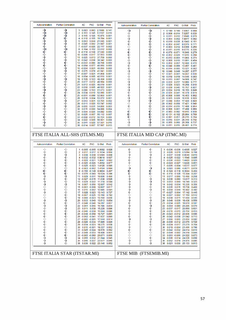
57

FTSE ITALIA ALL-SHS (ITLMS.MI) FTSE ITALIA MID CAP (ITMC.MI)

FTSE ITALIA STAR (ITSTAR.MI) FTSE MIB (FTSEMIB.MI)

58

Table 4.1.7 Serial Correlation of Weekly Indexes Returns

The serial correlation test performed casts light on weekly data nature. None of the indexes

show AC values equal to zero, but most of them are close to zero, especially in the first three

lags. There is absence of serial correlation, so there is no possibility to reject the null

hypothesis, a part for FTSE IT MICRO CAP that shows no reliable significance.

Monthly analysis

Descriptive Analysis

Hereunder there is the descriptive analysis of monthly data (Table 4.2.2). Indexes show both

negative and positive mean as before. Here, the highest mean is represented by the FTSE

ITALIA STAR index, while the lowest one by the FTSE IT SMALL CAP index. FTSE MIB,

FTSE IT ALL-SHS and FTSE IT SMALL CAP indexes, in order of size, show the highest

volatility compared with the others, proving a dispersion of data higher with respect to other

indexes. The FTSE IT MICRO CAP index proves itself again to be the less volatile index.

Skweness indicates that more than the half of the indexes present negative asymmetry, the

remaining ones positive asymmetry. Kurtosis highlights, with less power than daily and

weekly tests, that indexes are all centred with lights tails. Jarque-Bera test suggest that all

indexes could be part of a sample distributed such as a normal random variable. P-values are

59

significant at conventional level. So, results show the possibility that these indexes can be

represented by a normal distribution.

FTSE IT MICRO CAP

(ITMI.MI)

FTSE IT SMALL CAP

(ITSC.MI)

Mean -0.000533

Median -0.004399

Maximum 0.101259

Minimum -0.106699

Std. Dev. 0.042944

Skewness 0.002743

Kurtosis 2.557975

Jarque-Bera 0.586248

Probability 0.745929

Mean -0.003192

Median 0.001138

Maximum 0.153825

Minimum -0.167443

Std. Dev. 0.062911

Skewness -0.066219

Kurtosis 3.194997

Jarque-Bera 0.166691

Probability 0.920033

FTSE ITALIA ALL-SHS

(ITLMS.MI)

FTSE ITALIA MID CAP

(ITMC.MI)

Mean 0.000204

Median 0.001335

Maximum 0.175204

Minimum -0.150522

Std. Dev. 0.064445

Skewness -0.142062

Kurtosis 2.776273

Jarque-Bera 0.392341

Probability 0.821872

Mean 0.003156

Median 0.007948

Maximum 0.140468

Minimum -0.130417

Std. Dev. 0.052619

Skewness 0.067841

Kurtosis 2.613736

Jarque-Bera 0.502829

Probability 0.777700

FTSE ITALIA STAR

(ITSTAR.MI)

FTSE MIB

(FTSEMIB.MI)

Mean 0.010833

Median 0.013298

Maximum 0.143101

Minimum -0.109644

Std. Dev. 0.044428

Skewness -0.022868

Kurtosis 3.599380

Mean -0.000323

Median 0.001949

Maximum 0.188966

Minimum -0.169271

Std. Dev. 0.068631

Skewness -0.169041

Kurtosis 2.960027

60

Jarque-Bera 1.084045

Probability 0.581571

Jarque-Bera 0.347693

Probability 0.840426

Table 4.1.8 Descriptive Analysis of Monthly indexes returns

Runs test

ITMI.MI ITSC.MI ITLMS.MI ITMC.MI ITSTAR.MI FTSEMIB.MI

Z

P-value

Z

P-value

Z

P-value

Z

P-value

Z

P-

value

Z

P-value

-.95 .34 .47 .63 0 1 -.95 34 -.47 .63 0 1

Table 4.1.9 Runs Test for Monthly returns on Italian Stock Exchange indexes

All the indexes based on monthly data appear to follow a random process at the 5%

significance level. This means that – on the basis of the Runs test – all Italian indexes result

efficient looking at month by month opportunities.

Unit Root test

Augmented Dickey-Fuller Test

LEVEL

ITMI.MI ITSC.MI ITLMS.MI ITMC.MI ITSTAR.MI FTSEMIB.MI

t-Statistic -1.636714 -1.233176 -1.910166 -1.290406 -1.196992 -1.900363

Prob.* 0.4587 0.6558 0.3259 0.6298 0.6715 0.3304

TEST CRITICAL VALUE

1% level -3.527045 -3.525618 -3.525618 -3.525618 -3.527045 -3.525618

5% level -2.903566 -2.902953 -2.902953 -2.902953 -2.903566 -2.902953

10% level -2.589227 -2.588902 -2.588902 -2.588902 -2.589227 -2.588902

*MacKinnon (1996) one-sided p-values.

Table 4.2.0 ADF Test for Monthly indexes returns (level)

Results are smaller with respect to the critical values and the associated one-sided p-value

indicates that observations are consistent with the null hypothesis. This leads not to rejected

the null unit root hypothesis at conventional level. In other words, market indexes suggest the

presence of weak efficiency in the Italian market, even for FTSEMIB and ITLMS which show

higher value than the values of the other indexes. This is confirmed by the PP test below too.

61

Philip-Perron Test

LEVEL

ITMI.MI ITSC.MI ITLMS.MI ITMC.MI ITSTAR.MI FTSEMIB.MI

t-Statistic -1.478253 -1.327966 -1.887157 -1.467209 -0.736188 -1.853117

Prob.* 0.5389 0.6123 0.3365 0.5444 0.8303 0.3524

TEST CRITICAL VALUE

1% level -3.525618 -3.525618 -3.525618 -3.525618 -3.525618 -3.525618

5% level -2.902953 -2.902953 -2.902953 -2.902953 -2.902953 -2.902953

10% level -2.588902 -2.588902 -2.588902 -2.588902 -2.588902 -2.588902

*MacKinnon (1996) one-sided p-values.

Table 4.2.1 PP Test for Monthly indexes log prices (level)

Serial Correlation Test

FTSE IT MICRO CAP (ITMI.MI) FTSE IT SMALL CAP (ITSC.MI)

FTSE ITALIA ALL-SHS (ITLMS.MI) FTSE ITALIA MID CAP (ITMC.MI)

62

FTSE ITALIA STAR (ITSTAR.MI) FTSE MIB (FTSEMIB.MI)

Table 4.2.2 Serial Correlation of Monthly Indexes Returns

All data indexes show large p-values with significant Q-statistic results and autocorrelation

values close to zero. There is absence of serial correlation, and so the null hypothesis results

to be respected. Be careful, serial correlation test has been performed with log return data.

Companies Analysis

Purpose of the analysis on Companies: although the analysis over indexes looks at the whole

market, it is interesting to look at specific companies as well. If it could be proved that even

63

companies which form the market indexes are subjected to the efficient market hypothesis,

hence it is possible to affirm the EMH holds for the Italian market as whole.

4.1.4 Data

As done before for the indexes, now the first step in order to examine specific companies of

the Italian Market is defining data. Data collected for the study of the companies consist of

observations for the period January 1, 2009-December 31, 2014.

This empirical analysis of this study uses data of adjusted close prices for eight companies

quoted on the FTSE MIB index of the Italian Stock Exchange: BMPS (BANCA MONTE

PASCHI SIENA); ENEL.MI; ENI.MI; FNC.MI (FINMECCANICA); ISP.MI (INTESA SAN

PAOLO); MS.MI (MEDIASET); TIT.MI (TELECOM ITALIA); UCG.MI (UNICREDIT).

This companies have been chosen on the basis of their actual financial situation (especially to

observe the trends generated by BMPS), as well as the opportunity to look at big companies

operating in different industries. The choice comes from my personal belief that the behaviour

of these companies do not get too away from other companies of the FTSE MIB, indeed these

companies have a long existence, as well as being well renowned in the Country. Moreover

these companies did not enjoy merger and acquisition over time (i.e., FCA is not part of the

sample because trends would be distorted)

Index Notations Sample Period Observations

Daily Weekly Monthly

BANCA MONTE

PASCHI SIENA

BMPS

1/1/2009-

31/12/2014

1566 314 73

ENEL ENEL.MI 1/1/2009-

31/12/2014

1566 314 73

ENI ENI.MI 1/1/2009-

31/12/2014

1566 314 73

FINMECCANICA FNC.MI 1/1/2009-

31/12/2014

1566 314 73

INTESA SAN

PAOLO

ISP.MI 1/1/2009-

31/12/2014

1566 314

73

MEDIASET MS.MI 1/1/2009-

31/12/2014

1566 314 73

TELECOM TIT.MI 1/1/2009- 1566 314 73

64

Table 4.2.3 Description of Data Samples (Companies)

Hereinafter I drew companies graphs divided on the basis of days, weeks and months during

the six years above defined. Log prices are used in the analysis.

BMPS ENEL.MI

ENI.MI FNC.MI

ISP.MI MS.MI

UCG.MI TIT.MI

0.4

0.8

1.2

1.6

2.0

2.4

2.8

3.2

3.6

2009 2010 2011 2012 2013 2014

log price

0.7

0.8

0.9

1.0

1.1

1.2

1.3

1.4

1.5

1.6

2009 2010 2011 2012 2013 2014

Log Price

2.4

2.5

2.6

2.7

2.8

2.9

3.0

3.1

2009 2010 2011 2012 2013 2014

Log Price

0.8

1.2

1.6

2.0

2.4

2.8

2009 2010 2011 2012 2013 2014

Log Price

-0.2

0.0

0.2

0.4

0.6

0.8

1.0

1.2

2009 2010 2011 2012 2013 2014

Log Price

0.0

0.4

0.8

1.2

1.6

2.0

2009 2010 2011 2012 2013 2014

Log Price

ITALIA 31/12/2014

UNICREDIT UCG.MI 1/1/2009-

31/12/2014

1566 314 73

65

Table 4.2.4 Time Series Plots of Daily Prices of FTSE MIB Selected Companies

The daily graphic analysis leads to make some considerations. BMPS shows weak appearance

a negative trend that approximately starts in 2010 and causes a reliable slowdown in 2011.

Indeed it is well known what is the situation of the Bank nowadays. Other indexes, on the

other hand, suggest that the changes of trends are casual, and they appear to have permanent

effect on following values. This could mean there exist presence of unit roots in the time

series relatives to selected companies’ prices.

BMPS ENEL.MI

ENI.MI FNC.MI

ISP.MI MS.MI

0.4

0.8

1.2

1.6

2.0

2.4

2.8

3.2

2009 2010 2011 2012 2013 2014

Log price

-.8

-.6

-.4

-.2

.0

.2

.4

2009 2010 2011 2012 2013 2014

Log Price

0.5

1.0

1.5

2.0

2.5

3.0

3.5

4.0

2009 2010 2011 2012 2013 2014

Log Price

0.7

0.8

0.9

1.0

1.1

1.2

1.3

1.4

1.5

1.6

2009 2010 2011 2012 2013 2014

Log Price

2.4

2.5

2.6

2.7

2.8

2.9

3.0

3.1

2009 2010 2011 2012 2013 2014

Log Price

0.8

1.2

1.6

2.0

2.4

2.8

2009 2010 2011 2012 2013 2014

Log Price

66

UCG.MI TIT.MI

Table 4.2.5 Time Series Plots of Weekly Prices of FTSE MIB Selected Companies

BMPS ENEL.MI

ENI.MI FNC.MI

ISP.MI MS.MI

-0.2

0.0

0.2

0.4

0.6

0.8

1.0

1.2

2009 2010 2011 2012 2013 2014

Log Price

0.0

0.4

0.8

1.2

1.6

2.0

2009 2010 2011 2012 2013 2014

Log Price

0.8

1.2

1.6

2.0

2.4

2.8

3.2

2009 2010 2011 2012 2013 2014

Log Price

-.8

-.6

-.4

-.2

.0

.2

.4

2009 2010 2011 2012 2013 2014

Log Price

0.5

1.0

1.5

2.0

2.5

3.0

3.5

4.0

2009 2010 2011 2012 2013 2014

Log Price

0.8

0.9

1.0

1.1

1.2

1.3

1.4

1.5

1.6

2009 2010 2011 2012 2013 2014

Log Price

2.5

2.6

2.7

2.8

2.9

3.0

3.1

2009 2010 2011 2012 2013 2014

Log Price

0.8

1.2

1.6

2.0

2.4

2.8

2009 2010 2011 2012 2013 2014

Log Price

67

UCG.MI TIT.MI

Table 4.2.6 Time Series Plots of Monthly Prices of FTSE MIB Selected Companies

Although there are some differences, it is quite evident that daily, weekly and monthly data of

the same company show the same trend over time. It is remarkable to underline that Intesa

San Paolo does not show any trends in any timeline.

It is possible to examine companies’ trends looking at log returns.

BMPS ENEL.MI

ENI.MI FNC.MI

-0.2

0.0

0.2

0.4

0.6

0.8

1.0

1.2

2009 2010 2011 2012 2013 2014

Log Price

0.0

0.4

0.8

1.2

1.6

2.0

2009 2010 2011 2012 2013 2014

Log Price

0.8

1.2

1.6

2.0

2.4

2.8

2009 2010 2011 2012 2013 2014

Log Price

-.7

-.6

-.5

-.4

-.3

-.2

-.1

.0

.1

.2

2009 2010 2011 2012 2013 2014

Log Price

-.3

-.2

-.1

.0

.1

.2

2009 2010 2011 2012 2013 2014

log return

-.16

-.12

-.08

-.04

.00

.04

.08

2009 2010 2011 2012 2013 2014

Log Return

68

ISP.MI MS.MI

UCG.MI TIT.MI

Table 4.2.7 Time Series Plots of Daily Log Returns of FTSE MIB Selected Companies

BMPS ENEL.MI

ENI.MI FNC.MI

-.100

-.075

-.050

-.025

.000

.025

.050

.075

.100

2009 2010 2011 2012 2013 2014

Log Return

-.3

-.2

-.1

.0

.1

.2

2009 2010 2011 2012 2013 2014

Log Return

-.20

-.15

-.10

-.05

.00

.05

.10

.15

.20

2009 2010 2011 2012 2013 2014

Log Return

-.15

-.10

-.05

.00

.05

.10

.15

.20

2009 2010 2011 2012 2013 2014

Log Return

-.2

-.1

.0

.1

.2

2009 2010 2011 2012 2013 2014

Log Return

-.12

-.08

-.04

.00

.04

.08

.12

2009 2010 2011 2012 2013 2014

Log Return

-.4

-.3

-.2

-.1

.0

.1

.2

.3

.4

2009 2010 2011 2012 2013 2014

Log Return

-.20

-.15

-.10

-.05

.00

.05

.10

.15

2009 2010 2011 2012 2013 2014

Log Return

69

ISP.MI MS.MI

UCG.MI TIT.MI

Table 4.2.8 Time Series Plots of Weekly Log Returns of FTSE MIB Selected Companies

BMPS ENEL.MI

ENI.MI FNC.MI

-.25

-.20

-.15

-.10

-.05

.00

.05

.10

2009 2010 2011 2012 2013 2014

Log Return

-.3

-.2

-.1

.0

.1

.2

2009 2010 2011 2012 2013 2014

Log Return

-.3

-.2

-.1

.0

.1

.2

.3

2009 2010 2011 2012 2013 2014

Log Return

-.24

-.20

-.16

-.12

-.08

-.04

.00

.04

.08

.12

.16

2009 2010 2011 2012 2013 2014

Log Return

-.4

-.3

-.2

-.1

.0

.1

.2

.3

2009 2010 2011 2012 2013 2014

Log Return

-.15

-.10

-.05

.00

.05

.10

.15

.20

.25

2009 2010 2011 2012 2013 2014

Log Return

-.6

-.4

-.2

.0

.2

.4

.6

2009 2010 2011 2012 2013 2014

Log Return

-.16

-.12

-.08

-.04

.00

.04

.08

.12

.16

2009 2010 2011 2012 2013 2014

Log Return

70

ISP.MI MS.MI

UCG.MI TIT.MI

Table 4.2.9 Time Series Plots of Monthly Log Returns of FTSE MIB Selected Companies

It appears evident the presence of an high level of volatility affecting all the companies

selected, more or less at the same level.

4.1.5 Weak Hypothesis

{𝐻0: 𝑇ℎ𝑒 𝐼𝑡𝑎𝑙𝑖𝑎𝑛 𝑆𝑡𝑜𝑐𝑘 𝑀𝑎𝑟𝑘𝑒𝑡 𝑖𝑠 𝑤𝑒𝑎𝑘 − 𝑓𝑜𝑟𝑚 𝑒𝑓𝑓𝑖𝑐𝑖𝑒𝑛𝑡

𝐻1: 𝑇ℎ𝑒 𝐼𝑡𝑎𝑙𝑖𝑎𝑛 𝑆𝑡𝑜𝑐𝑘 𝑀𝑎𝑟𝑘𝑒𝑡 𝑑𝑜𝑒𝑠 𝑛𝑜𝑡 𝑓𝑜𝑙𝑙𝑜𝑤 𝑎 𝑟𝑎𝑛𝑑𝑜𝑚 𝑤𝑎𝑙𝑘

-.15

-.10

-.05

.00

.05

.10

.15

.20

2009 2010 2011 2012 2013 2014

Log Return

-.5

-.4

-.3

-.2

-.1

.0

.1

.2

2009 2010 2011 2012 2013 2014

Log Return

-.3

-.2

-.1

.0

.1

.2

.3

2009 2010 2011 2012 2013 2014

Log Return

-.4

-.3

-.2

-.1

.0

.1

.2

.3

2009 2010 2011 2012 2013 2014

Log Return

-.4

-.3

-.2

-.1

.0

.1

.2

.3

.4

2009 2010 2011 2012 2013 2014

Log Return

-.3

-.2

-.1

.0

.1

.2

2009 2010 2011 2012 2013 2014

Log Return

71

4.1.6 Methodology and Results

In order to verify the hypothesis above, it has been used some statistical methods: descriptive

analysis; the serial correlation test; the runs test; the sign test; the Augmented Dickey-Fuller

and the Phillips-Perron unit root tests. In the following part it is possible to appreciate results

of the analysis:

Daily analysis

Descriptive Analysis

BMPS ENEL.MI

Mean 13.22980

Median 8.170000

Maximum 33.73470

Minimum 1.888100

Std. Dev. 9.011182

Skewness 0.524339

Kurtosis 1.744747

Jarque-Bera 174.5688

Probability 0.000000

Mean 3.521919

Median 3.669000

Maximum 4.832000

Minimum 2.034000

Std. Dev. 0.623629

Skewness -0.247208

Kurtosis 2.018937

Jarque-Bera 78.75230

Probability 0.000000

ENI.MI FNC.MI

Mean 16.91433

Median 17.10000

Maximum 20.41000

Minimum 12.17000

Std. Dev. 1.319303

Skewness -0.609348

Kurtosis 3.998725

Jarque-Bera 161.9942

Probability 0.000000

Mean 6.966502

Median 7.052500

Maximum 12.72000

Minimum 2.620000

Std. Dev. 2.773127

Skewness 0.115006

Kurtosis 1.736534

Jarque-Bera 107.6137

Probability 0.000000

ISP.MI MS.MI

Mean 1.899712

Median 1.993200

Maximum 3.003600

Minimum 0.868000

Std. Dev. 0.545722

Skewness -0.016783

Kurtosis 1.817425

Mean 3.447743

Median 3.446000

Maximum 6.485000

Minimum 1.166000

Std. Dev. 1.309733

Skewness 0.051758

Kurtosis 2.091111

72

Jarque-Bera 91.32456

Probability 0.000000

Jarque-Bera 54.60088

Probability 0.000000

UCG.MI TIT.MI

Mean 7.543875

Median 5.898750

Maximum 16.78220

Minimum 2.204400

Std. Dev. 3.942104

Skewness 0.535372

Kurtosis 1.906951

Jarque-Bera 152.7663

Probability 0.000000

Mean 0.877705

Median 0.882500

Maximum 1.253000

Minimum 0.471000

Std. Dev. 0.168754

Skewness -0.287508

Kurtosis 2.387494

Jarque-Bera 46.05394

Probability 0.000000

Table 4.3.0 Descriptive Analysis of Daily Companies Returns

The descriptive analysis of the selected companies, on the basis of the daily returns,

underlines that half companies show negative mean and half present a positive one. MS.MI

represents the highest mean among these companies, while UCG.MI has the lowest one.

Results from standard deviations confirm the hypothesis of high volatility made before. ENI

and Finmeccanica seem to be the companies with most dispersion of returns with respect to

their mean, whereas Telecom Italia presents the lowest standard deviation value, so the lowest

volatility among the selected sample. Finmeccanica, Intesa San Paolo and Telecom Italia

presents negative value for skewness. Moreover Mediaset, Banca Monte Paschi di Siena and

Intesa San Paolo are centred stronger than the other observed companies. Jarque-Bera test

suggest that the most part of the companies have been extracted by a sample not distributed

such as a normal random variable, a part from a weak result concerning Finmeccanica.

FNC.MI is also the only company to show significance on the basis of a p-value of 0.848705.

Results suggest the only company that could be represented by a normal distribution would be

Finmeccanica, but it does not appear to reach all the owed properties.

Runs test

Now it is possible to look at runs test result for companies daily returns as well:

BMPS.MI ENEL.MI ENI.MI FNC.MI ISP.MI MS.MI UCG.MI TIT.MI

Z P-

value Z

P-

value Z

P-

value Z

P-

value Z

P-

value Z

P-

value Z

P-

value Z

P-

value

73

-2.28 .02 1.93 .05 1.14 .25 .28 .78 1.36 .17 -2.01 .04 .12 .9 .08 .94

Table 4.3.1 Runs Test for Daily returns on FTSE MIB Selected Companies

BMPS, MS.MI and TIT.MI are the only companies that seem not to follow some randomness

processes, but first two cited companies show dat not really significance. By the way, this

leads to think that the other companies are supposed to be efficient under the weak form.

Unit Root test

In order to join more reliable results, ADF and PP tests, with their relatives first differences,

have been performed. These tests are based on log prices.

Augmented Dickey-Fuller Test

LEVEL

BMPS.MI ENEL.MI ENI.MI FNC.MI ISP.MI MS.MI UCG.MI TIT.MI

t-Statistic -0.392914 -2.041856 -3.711379 -1.444246 -1.884979 -1.247856 -1.389292 -2.366591

Prob.* 0.9080 0.2689 0.0041 0.5617 0.3396 0.6555 0.5890 0.1515

TEST CRITICAL VALUE

1% level -3.434325 -3.434323 -3.434323 -3.434323 -3.434323 -3.434323 -3.434325 -3.434323

5% level -2.863183 -2.863182 -2.863182 -2.863182 -2.863182 -2.863182 -2.863183 -2.863182

10% level -2.567693 -2.567692 -2.567692 -2.567692 -2.567692 -2.567692 -2.567693 -2.567692

*MacKinnon (1996) one-sided p-values.

Table 4.3.2 ADF Test for Daily FTSE MIB Selected Companies (level)

Here, there is something that immediately appears evident, ENI is on the left of the critical

values. This leads to think that ENI does not appear weak efficient considering daily prices.

The result could be an open door for investors in order to beat the market. By the way, p-

value over ENI’s results does not lead to any significant levels. Remains the fact that result

for ENI suggest the absence of a unit root, so the rejection of the null hypothesis. Moreover,

also Telecom appears to be weakly smaller than its critical values.

Philip-Perron Test

LEVEL

BMPS.MI ENEL.MI ENI.MI FNC.MI ISP.MI MS.MI UCG.MI TIT.MI

t-Statistic -0.249340 -1.993124 -3.813543 -1.463946 -1.688596 -1.264650 -1.320413 -2.236335

74

Prob.* 0.9296 0.2900 0.0028 0.5519 0.4369 0.6479 0.6220 0.1935

TEST CRITICAL VALUE

1% level -3.434323 -3.434323 -3.434323 -3.434323 -3.434323 -3.434323 -3.434323 -3.434323

5% level -2.863182 -2.863182 -2.863182 -2.863182 -2.863182 -2.863182 -2.863182 -2.863182

10% level -2.567692 -2.567692 -2.567692 -2.567692 -2.567692 -2.567692 -2.567692 -2.567692

*MacKinnon (1996) one-sided p-values.

Table 4.3.3 PP Test for Daily FTSE MIB Selected Companies (level)

The PP leads exactly to the same results of the ADF test.

Serial Correlation Test

{

𝐻0: 𝐷𝑎𝑡𝑎 𝑎𝑟𝑒 𝑖𝑛𝑑𝑒𝑝𝑒𝑛𝑑𝑒𝑛𝑡𝑙𝑦 𝑑𝑖𝑠𝑡𝑟𝑖𝑏𝑢𝑡𝑒𝑑 (𝑡ℎ𝑒 𝑐𝑜𝑟𝑟𝑒𝑙𝑎𝑡𝑖𝑜𝑛𝑠 𝑎𝑟𝑒 𝑒𝑞𝑢𝑎𝑙 𝑡𝑜 𝑧𝑒𝑟𝑜, 𝑠𝑜 𝑎𝑛𝑦 𝑜𝑏𝑠𝑒𝑟𝑣𝑒𝑑 𝑐𝑜𝑟𝑟𝑒𝑙𝑎𝑡𝑖𝑜𝑛𝑠 𝑟𝑒𝑠𝑖𝑙𝑡 𝑓𝑟𝑜𝑚 𝑟𝑎𝑛𝑑𝑜𝑚𝑛𝑒𝑠𝑠)

𝐻1: 𝑇ℎ𝑒 𝑑𝑎𝑡𝑎 𝑎𝑟𝑒 𝑛𝑜𝑡 𝑖𝑛𝑑𝑒𝑝𝑒𝑛𝑑𝑒𝑛𝑡𝑙𝑦 𝑑𝑖𝑠𝑡𝑟𝑖𝑏𝑢𝑡𝑒𝑑 (𝑠𝑒𝑟𝑖𝑎𝑙 𝑐𝑜𝑟𝑟𝑒𝑙𝑎𝑡𝑖𝑜𝑛)

It is helpful to repeat that no serial correlation in residuals means that the autocorrelations and

partial autocorrelations at all lags should be nearly zero, and all Q-statistics should be

insignificant with large p-values. The Ljung-Box test has been carried out on the basis of log

return data.

BMPS ENEL.MI

75

ENI.MI FNC.MI

ISP.MI MS.MI

UCG.MI TIT.MI

76

Table 4.3.4 Serial Correlation of Daily FTSE MIB Selected Companies

A part for BMPS and UCG companies show some low p-values, leading to reject the absence

of serial correlation, and so the null hypothesis, if considered with the AC and PAC value

which differ from zero (even if really close to it). On the other hand, almost all the companies

do not reject the null hypothesis and so are consistent with the efficient market hypothesis.

Weekly analysis

Descriptive Analysis

BMPS ENEL.MI

Mean 13.23605

Median 8.143300

Maximum 32.96120

Minimum 1.912500

Std. Dev. 9.053442

Skewness 0.519649

Kurtosis 1.736595

Jarque-Bera 35.01534

Mean 3.526465

Median 3.686500

Maximum 4.832000

Minimum 2.180000

Std. Dev. 0.625748

Skewness -0.255377

Kurtosis 2.040991

Jarque-Bera 15.44576

77

Probability 0.000000

Probability 0.000443

ENI.MI FNC.MI

Mean 16.92000

Median 17.11000

Maximum 20.41000

Minimum 12.20000

Std. Dev. 1.304258

Skewness -0.553892

Kurtosis 4.087784

Jarque-Bera 31.53682

Probability 0.000000

Mean 6.972296

Median 7.075000

Maximum 12.67000

Minimum 2.678000

Std. Dev. 2.778483

Skewness 0.113001

Kurtosis 1.740975

Jarque-Bera 21.40722

Probability 0.000022

ISP.MI MS.MI

Mean 1.902262

Median 2.001200

Maximum 3.003600

Minimum 0.938000

Std. Dev. 0.543226

Skewness -0.030356

Kurtosis 1.817917

Jarque-Bera 18.32985

Probability 0.000105

Mean 3.450897

Median 3.463000

Maximum 6.415000

Minimum 1.197000

Std. Dev. 1.311780

Skewness 0.048622

Kurtosis 2.091260

Jarque-Bera 10.92806

Probability 0.004236

UCG.MI TIT.MI

Mean 7.545173

Median 5.883450

Maximum 16.78220

Minimum 2.335600

Std. Dev. 3.934684

Skewness 0.533833

Kurtosis 1.906341

Jarque-Bera 30.56267

Probability 0.000000

Mean 0.878432

Median 0.880000

Maximum 1.251000

Minimum 0.476700

Std. Dev. 0.168408

Skewness -0.300358

Kurtosis 2.377461

Jarque-Bera 9.791765

Probability 0.007477

Table 4.3.5 Descriptive Analysis of Weekly FTSE MIB Selected Companies

The descriptive analysis of the selected companies, on the basis of the weekly returns,

highlights the clear contrast from BMPS.MI to UCG.MI in terms of mean. The daily returns

high volatility is confirmed by weekly evidences too. ENI and Finmeccanica again with most

dispersion than others. Moreover Mediaset, Banca Monte Paschi di Siena, Unicredit and

Intesa San Paolo are centred stronger than the other observed companies. Jarque-Bera test

78

suggest that the most part of the companies have been extracted by a sample not distributed

such as a normal random variable. FNC.MI confirms to be an exception.

Runs Test

BMPS ENEL.MI ENI.MI FNC.MI ISP.MI MS.MI UCG.MI TIT.MI

Z P-

value Z

P-

value Z

P-

value Z

P-

value Z

P-

value Z

P-

value Z

P-

value Z

P-

value

.11 .91 -.23 .82 -.11 .91 .9 .37 0 1 -1.58 .11 .34 .73 1.13 .26

Table 4.3.6 Runs Test for Weekly returns on FTSE MIB Selected Companies

All companies appear to follow a random order process. Hence, for what concerns weekly

analysis, the whole selected sample of campanies appear to be weak form efficient.

Unit Root test

Augmented Dickey-Fuller Test

LEVEL

BMPS.MI ENEL.MI ENI.MI FNC.MI ISP.MI MS.MI UCG.MI TIT.MI

t-Statistic -0.205830 -1.964814 -3.766310 -1.454239 -1.747778 -1.237516 -1.250745 -2.289314

Prob.* 0.9347 0.3025 0.0036 0.5556 0.4062 0.6589 0.6530 0.1761

TEST CRITICAL VALUE

1% level -3.451078 -3.451078 -3.451078 -3.451078 -3.451078 -3.451078 -3.451078 -3.451078

5% level -2.870561 -2.870561 -2.870561 -2.870561 -2.870561 -2.870561 -2.870561 -2.870561

10% level -2.571647 -2.571647 -2.571647 -2.571647 -2.571647 -2.571647 -2.571647 -2.571647

*MacKinnon (1996) one-sided p-values.

Table 4.3.7 ADF Test for Weekly FTSE MIB Selected Companies (level)

Philip-Perron Test

LEVEL

BMPS.MI ENEL.MI ENI.MI FNC.MI ISP.MI MS.MI UCG.MI TIT.MI

t-Statistic -0.245977 -2.012348 -3.726090 -1.561244 -1.678354 -1.363130 -1.279372 -2.113676

Prob.* 0.9294 0.2815 0.0042 0.5012 0.4413 0.6005 0.6400 0.2395

TEST CRITICAL VALUE

1% level -3.451078 -3.451078 -3.451078 -3.451078 -3.451078 -3.451078 -3.451078 -3.451078

5% level -2.870561 -2.870561 -2.870561 -2.870561 -2.870561 -2.870561 -2.870561 -2.870561

10% level -2.571647 -2.571647 -2.571647 -2.571647 -2.571647 -2.571647 -2.571647 -2.571647

*MacKinnon (1996) one-sided p-values.

Table 4.3.8 PP Test for Weekly FTSE MIB Selected Companies (level)

79

Again, weekly data show positive results to confirm the null hypothesis for all the company

selected but ENI.

Serial Correlation Test

BMPS ENEL.MI

ENI.MI FNC.MI

80

ISP.MI MS.MI

UCG.MI TIT.MI

81

Table 4.3.9 Serial Correlation of Weekly FTSE MIB Selected Companies

Weekly data tested for serial correlation confirm the companies selected cannot be identify in

a random process, but the results lead to suppose an approximation to the random walk exists,

and so there exist the possibility of presence of weak form efficiency too.

Monthly analysis

Descriptive Analysis

BMPS ENEL.MI

Mean 13.24745

Median 8.131900

Maximum 32.78930

Minimum 1.912500

Std. Dev. 9.154201

Skewness 0.521662

Kurtosis 1.764007

Jarque-Bera 7.957619

Probability 0.018708

Mean 3.529714

Median 3.680000

Maximum 4.816000

Minimum 2.298000

Std. Dev. 0.625372

Skewness -0.198198

Kurtosis 2.106198

Jarque-Bera 2.907869

Probability 0.233649

ENI.MI FNC.MI

82

Mean 16.89986

Median 17.00000

Maximum 20.10000

Minimum 13.02000

Std. Dev. 1.269989

Skewness -0.478323

Kurtosis 3.489197

Jarque-Bera 3.511554

Probability 0.172773

Mean 6.997973

Median 7.025000

Maximum 12.13000

Minimum 2.728000

Std. Dev. 2.793289

Skewness 0.096703

Kurtosis 1.664729

Jarque-Bera 5.536911

Probability 0.062759

ISP.MI MS.MI

Mean 1.908696

Median 1.952000

Maximum 2.954300

Minimum 0.997500

Std. Dev. 0.539197

Skewness -0.070197

Kurtosis 1.720163

Jarque-Bera 5.042147

Probability 0.080373

Mean 3.456899

Median 3.440000

Maximum 6.415000

Minimum 1.214000

Std. Dev. 1.319629

Skewness 0.073947

Kurtosis 2.152369

Jarque-Bera 2.251899

Probability 0.324344

UCG.MI TIT.MI

Mean 7.511841

Median 6.021000

Maximum 15.75130

Minimum 2.408900

Std. Dev. 3.878725

Skewness 0.520571

Kurtosis 1.853851

Jarque-Bera 7.292801

Probability 0.026085

Mean 0.882500

Median 0.891000

Maximum 1.150000

Minimum 0.512500

Std. Dev. 0.169978

Skewness -0.378028

Kurtosis 2.277711

Jarque-Bera 3.325522

Probability 0.189615

Table 4.4.0 Descriptive Analysis of Monthly Companies Returns

It is evident that monthly observation suggest more for normality. P-values suggest more

significance in results but standard deviations confirm a tendency of almost all companies to

suffer a certain volatility. Distributions also appear to be less centred than observed in the

previous examinations.

Runs test

83

BMPS ENEL.MI ENI.MI FNC.MI ISP.MI MS.MI UCG.MI TIT.MI

Z P-

value Z

P-

value Z

P-

value Z

P-

value Z

P-

value Z

P-

value Z

P-

value Z

P-

value

.12 .9 -1.06 .29 -.12 .91 -.59 .56 .59 .55 -.82 .41 -.59 .56 .12 .9

Table 4.4.1 Runs Test for Monthly returns on FTSE MIB Selected Companies

Monthly analysis gives back same results as weekly gave before. This means all companies

are supposed to be weak form efficient.

Unit Root test

Augmented Dickey-Fuller Test

LEVEL

BMPS.MI ENEL.MI ENI.MI FNC.MI ISP.MI MS.MI UCG.MI TIT.MI

t-Statistic -0.104127 -1.778844 -3.054587 -1.432481 -1.608144 -1.253222 -1.174932 -1.992398

Prob.* 0.9444 0.3880 0.0347 0.5618 0.4733 0.6469 0.6811 0.2896

TEST CRITICAL VALUE

1% level -3.524233 -3.524233 -3.524233 -3.524233 -3.524233 -3.524233 -3.524233 -3.524233

5% level -2.902358 -2.902358 -2.902358 -2.902358 -2.902358 -2.902358 -2.902358 -2.902358

10% level -2.588587 -2.588587 -2.588587 -2.588587 -2.588587 -2.588587 -2.588587 -2.588587

*MacKinnon (1996) one-sided p-values.

Table 4.4.2 ADF Test for Monthly FTSE MIB Selected Companies (level)

Philip-Perron Test

LEVEL

BMPS.MI ENEL.MI ENI.MI FNC.MI ISP.MI MS.MI UCG.MI TIT.MI

t-Statistic -0.179464 -1.929321 -3.250374 -1.432481 -1.569088 -1.302700 -1.258365 -1.904737

Prob.* 0.9355 0.3173 0.0211 0.5618 0.4931 0.6242 0.6446 0.3284

TEST CRITICAL VALUE

1% level -3.524233 -3.524233 -3.524233 -3.524233 -3.524233 -3.524233 -3.524233 -3.524233

5% level -2.902358 -2.902358 -2.902358 -2.902358 -2.902358 -2.902358 -2.902358 -2.902358

10% level -2.588587 -2.588587 -2.588587 -2.588587 -2.588587 -2.588587 -2.588587 -2.588587

*MacKinnon (1996) one-sided p-values.

Table 4.4.3 PP Test for Monthly FTSE MIB Selected Companies (level)

Monthly data seem to suggest more tendency not to refuse the null hypothesis with respect

both to daily and weekly ones. Indeed, ENI shows weak efficiency at 1% significant level on

the basis of the MacKinnon one-sided p-values.

84

Serial Correlation Test

Even monthly data give back results similar to the previous ones, excluding a strongly existence of

weak form efficiency into selected companies.

Finally the analysis to test the weak-form efficiency focuses on two anomalies established

during years: the day of the week effect and the January effect.

The Day Of The Week Effect

The most violations of the efficient market hypothesis have been identified in calendar

anomalies. Hereinafter will be examined the day of the week effect for each Italian Stock

Exchange index. Be a matter of days, it follows that the object of the examination are the

daily returns for the whole period of mine investigation (2009-2014). The purpose is to find

out whether there is any statistical significant difference among index returns on different

days of the week.

The starting point would be the following regression:

𝑅𝑡 = 𝜇 + 𝑏2𝐷2 + 𝑏3𝐷3 + 𝑏4𝐷4 + 𝑏5𝐷5 + 휀𝑡 (31)

where 𝐷1 is the dummy variable for Tuesday (that means 𝐷1 = 1 if the observation is on

Monday, 𝐷1 = 0 otherwise), 𝐷2 is the dummy variable for Wednesday, 𝐷3 is the dummy

variable for Thursday, and finally 𝐷4 is the dummy variable for Friday. The intercept 𝜇

represents the rate of change of Monday, while 𝑏𝑛 is the difference between the average rate

of daily change and 𝜇. The null hypothesis is the following:

𝐻0: 𝑏1 = 𝑏2 = 𝑏3 = 𝑏4 = 0

So the index will be proved subjected to the weak-form efficiency whether coefficient will

result equal to zero, otherwise the null hypothesis would not be proved consistent with the

data.

85

Now let’s see in the deep how each index behaves:

FTSE IT MICRO CAP

Dependent Variable: LOG_RETURNS

Method: Least Squares

Sample: 1/05/2009 12/30/2014

Included observations: 1519

Variable Coefficient Std. Error t-Statistic Prob.

@WEEKDAY=2 9.39E-05 0.000642 0.146288 0.8837

@WEEKDAY=3 -0.000307 0.000643 -0.477448 0.6331

@WEEKDAY=4 -0.000463 0.000643 -0.720526 0.4713

@WEEKDAY=5 0.000814 0.000646 1.260045 0.2078

C -5.00E-05 0.000456 -0.109635 0.9127

R-squared 0.003098 Mean dependent var -2.53E-05

Adjusted R-squared 0.000464 S.D. dependent var 0.007917

S.E. of regression 0.007915 Akaike info criterion -6.836798

Sum squared resid 0.094851 Schwarz criterion -6.819267

Log likelihood 5197.548 Hannan-Quinn criter. -6.830271

F-statistic 1.176099 Durbin-Watson stat 1.973705

Prob(F-statistic) 0.319464

Table 4.4.4 Day of the Week FTSE IT MICRO CAP

FTSE IT SMALL CAP

Dependent Variable: LOG_RETURNS

Method: Least Squares

Sample: 1/02/2009 12/30/2014

Included observations: 1520

Variable Coefficient Std. Error t-Statistic Prob.

@WEEKDAY=2 -0.000567 0.000973 -0.582465 0.5603

@WEEKDAY=3 0.000392 0.000974 0.402608 0.6873

@WEEKDAY=4 -0.000935 0.000974 -0.960794 0.3368

@WEEKDAY=5 -0.000700 0.000978 -0.716457 0.4738

C 0.000212 0.000691 0.306028 0.7596

R-squared 0.001654 Mean dependent var -0.000151

Adjusted R-squared -0.000982 S.D. dependent var 0.011987

S.E. of regression 0.011993 Akaike info criterion -6.005779

86

Sum squared resid 0.217889 Schwarz criterion -5.988258

Log likelihood 4569.392 Hannan-Quinn criter. -5.999256

F-statistic 0.627327 Durbin-Watson stat 1.611672

Prob(F-statistic) 0.643045

Table 4.4.5 Day of the Week FTSE IT SMALL CAP

FTSE IT ALL-SHS

Dependent Variable: LOG_RETURNS

Method: Least Squares

Sample: 1/02/2009 12/30/2014

Included observations: 1520

Variable Coefficient Std. Error t-Statistic Prob.

@WEEKDAY=2 0.002333 0.001310 1.781403 0.0750

@WEEKDAY=3 0.002804 0.001312 2.137177 0.0327

@WEEKDAY=4 0.001898 0.001311 1.447882 0.1479

@WEEKDAY=5 0.001692 0.001316 1.285152 0.1989

C -0.001741 0.000931 -1.870898 0.0616

R-squared 0.003463 Mean dependent var 9.64E-06

Adjusted R-squared 0.000832 S.D. dependent var 0.016156

S.E. of regression 0.016149 Akaike info criterion -5.410658

Sum squared resid 0.395087 Schwarz criterion -5.393137

Log likelihood 4117.100 Hannan-Quinn criter. -5.404135

F-statistic 1.316142 Durbin-Watson stat 1.976480

Prob(F-statistic) 0.261748

Table 4.4.6 Day of the Week FTSE IT ALL-SHS CAP

FTSE IT MID CAP

Dependent Variable: LOG_RETURNS

Method: Least Squares

Sample: 1/02/2009 12/30/2014

Included observations: 1520

Variable Coefficient Std. Error t-Statistic Prob.

@WEEKDAY=2 0.001059 0.001059 0.999494 0.3177

@WEEKDAY=3 0.001793 0.001061 1.690432 0.0912

@WEEKDAY=4 0.001704 0.001060 1.607391 0.1082

@WEEKDAY=5 0.001671 0.001064 1.569929 0.1166

87

C -0.001098 0.000753 -1.458998 0.1448

R-squared 0.002656 Mean dependent var 0.000149

Adjusted R-squared 0.000023 S.D. dependent var 0.013058

S.E. of regression 0.013058 Akaike info criterion -5.835595

Sum squared resid 0.258312 Schwarz criterion -5.818074

Log likelihood 4440.052 Hannan-Quinn criter. -5.829072

F-statistic 1.008753 Durbin-Watson stat 1.856060

Prob(F-statistic) 0.401651

Table 4.4.7 Day of the Week FTSE IT MID CAP

FTSE ITALIA STAR

Dependent Variable: LOG_RETURNS

Method: Least Squares

Sample: 1/02/2009 12/30/2014

Included observations: 1548

Variable Coefficient Std. Error t-Statistic Prob.

@WEEKDAY=2 0.002310 0.001368 1.688386 0.0915

@WEEKDAY=3 0.002814 0.001372 2.050137 0.0405

@WEEKDAY=4 0.001876 0.001372 1.367162 0.1718

@WEEKDAY=5 0.001593 0.001371 1.161814 0.2455

C -0.001732 0.000968 -1.788810 0.0738

R-squared 0.003124 Mean dependent var -1.50E-05

Adjusted R-squared 0.000540 S.D. dependent var 0.017078

S.E. of regression 0.017073 Akaike info criterion -5.299419

Sum squared resid 0.449762 Schwarz criterion -5.282156

Log likelihood 4106.750 Hannan-Quinn criter. -5.292998

F-statistic 1.208892 Durbin-Watson stat 1.989917

Prob(F-statistic) 0.305067

Table 4.4.8 Day of the Week FTSE ITALIA STAR

FTSE MIB

Dependent Variable: LOG_RETURNS

Method: Least Squares

Sample: 1/02/2009 12/30/2014

Included observations: 1548

Variable Coefficient Std. Error t-Statistic Prob.

@WEEKDAY=2 0.008162 0.025134 0.324731 0.7454

88

@WEEKDAY=3 0.008666 0.025215 0.343670 0.7311

@WEEKDAY=4 0.037988 0.025215 1.506538 0.1321

@WEEKDAY=5 0.001167 0.025195 0.046320 0.9631

C -0.007584 0.017787 -0.426376 0.6699

R-squared 0.001946 Mean dependent var 0.003577

Adjusted R-squared -0.000641 S.D. dependent var 0.313571

S.E. of regression 0.313671 Akaike info criterion 0.522282

Sum squared resid 151.8152 Schwarz criterion 0.539545

Log likelihood -399.2461 Hannan-Quinn criter. 0.528703

F-statistic 0.752084 Durbin-Watson stat 2.003083

Prob(F-statistic) 0.556596

Table 4.4.9 Day of the Week FTSE MIB

It is possible to look at the summarised results below:

Index 𝜇 Prob. 𝐷2 Prob. 𝐷3 Prob. 𝐷4 Prob. 𝐷5 Prob.

ITMI.MI -0.00005 0.9127 0.0000939 0.8837 -0.000307 0.6331 -0.000463 0.4713 0.000814 0.2078

ITSC.MI 0.000212 0.7596 -0.000567 0.5603 0.000392 0.6873 -0.000935 0.3368 -0.000700 0.4738

ITLMS.MI -0.001741 0.0616 0.002333 0.0750 0.002804 0.0327 0.001898 0.1479 0.001692 0.1989

ITMC.MI -0.001098 0.1448 0.001059 0.3177 0.001793 0.0912 0.001704 0.1082 0.001671 0.1166

ITSTAR.MI -0.001732 0.0738 0.002310 0.0915 0.002814 0.0405 0.001876 0.1718 0.001593 0.2455

FTSEMIB.MI -0.007584 0.6699 0.008162 0.7454 0.008666 0.7311 0.037988 0.1321 0.001167 0.9631

Table 4.5.0 Italian Stock Exchange Day of the week effect

It appears clear that none of the indexes present coefficients equal to zero, but they are all

close to it. Monday rates appears different from each other, furthermore they result negative, a

part for the FTSE IT SMALL CAP index. The fact that results show values close to zero, with

p-value that suggest as a good probability for those coefficients to be zero, allows not to reject

the null hypothesis. Hence all the indexes could be considered efficient under the weak

efficient form.

Index F-statistic Prob (F-statistic)

ITMI.MI 1.176099 0.319464

ITSC.MI 0.627327 0.643045

ITLMS.MI 1.316142 0.261748

ITMC.MI 1.008753 0.401651

ITSTAR.MI 1.208892 0.305067

FTSEMIB.MI 0.752084 0.556596

Table 4.5.1 Italian Stock Exchange Day of the week effect

89

In order to assess, easier and for sure, the proof of the weak efficiency under the day of the

week effect, the above table summarise results for the F-statistic and their relatives p-values.

Thanks to p-values it is easy to notice that F-statistics suggest all the indexes are efficient

under the weak-form. Indeed probabilities show value higher than the 𝛼. This means that all

indexes appear to follow a RW at 5% significance level.

The January Effect

Another important effect, as it has possible to see in the present work, is the January effect. In

order to test the presence of this effect into the Italian market, it has been performed a

regression as follow:

𝑅𝑡 = 𝜇 + 𝛽′𝐷𝑡 + 휀𝑡 (32)

Where 𝐷𝑡 is a dummy for the month of January34

.

Now, let’s proceed:

FTSE IT MICRO CAP

Dependent Variable: LOG_RETURNS

Method: Least Squares

Sample: 2009M01 2014M12

Included observations: 72

Variable Coefficient Std. Error t-Statistic Prob.

JANUARY 0.005325 0.018431 0.288899 0.7735

C -0.000977 0.005321 -0.183545 0.8549

R-squared 0.001191 Mean dependent var -0.000533

Adjusted R-squared -0.013078 S.D. dependent var 0.042944

S.E. of regression 0.043224 Akaike info criterion -3.417448

Sum squared resid 0.130783 Schwarz criterion -3.354208

Log likelihood 125.0281 Hannan-Quinn criter. -3.392272

F-statistic 0.083463 Durbin-Watson stat 1.474034

Prob(F-statistic) 0.773512

34

Data consist of monthly returns

90

Table 4.5.2 January effect FTSE IT MICRO CAP

FTSE IT SMALL CAP

Dependent Variable: LOG_RETURNS

Method: Least Squares

Sample: 2009M01 2014M12

Included observations: 72

Variable Coefficient Std. Error t-Statistic Prob.

JANUARY 0.039244 0.026606 1.475016 0.1447

C -0.006462 0.007680 -0.841367 0.4030

R-squared 0.030144 Mean dependent var -0.003192

Adjusted R-squared 0.016289 S.D. dependent var 0.062911

S.E. of regression 0.062397 Akaike info criterion -2.683229

Sum squared resid 0.272533 Schwarz criterion -2.619988

Log likelihood 98.59624 Hannan-Quinn criter. -2.658052

F-statistic 2.175671 Durbin-Watson stat 1.742760

Prob(F-statistic) 0.144692

Table 4.5.3 January effect FTSE IT SMALL CAP

FTSE IT ALL-SHS

Dependent Variable: LOG_RETURNS

Method: Least Squares

Sample: 2009M01 2014M12

Included observations: 72

Variable Coefficient Std. Error t-Statistic Prob.

JANUARY 0.016954 0.027601 0.614262 0.5410

C -0.001209 0.007968 -0.151773 0.8798

R-squared 0.005361 Mean dependent var 0.000204

Adjusted R-squared -0.008848 S.D. dependent var 0.064445

S.E. of regression 0.064730 Akaike info criterion -2.609811

Sum squared resid 0.293295 Schwarz criterion -2.546570

Log likelihood 95.95318 Hannan-Quinn criter. -2.584634

F-statistic 0.377318 Durbin-Watson stat 1.826567

Prob(F-statistic) 0.541034

Table 4.5.4 January effect FTSE IT ALL-SHS

FTSE IT MID CAP

91

Dependent Variable: LOG_RETURNS

Method: Least Squares

Sample: 2009M01 2014M12

Included observations: 72

Variable Coefficient Std. Error t-Statistic Prob.

JANUARY 0.029832 0.022313 1.336952 0.1856

C 0.000670 0.006441 0.104031 0.9174

R-squared 0.024899 Mean dependent var 0.003156

Adjusted R-squared 0.010969 S.D. dependent var 0.052619

S.E. of regression 0.052329 Akaike info criterion -3.035136

Sum squared resid 0.191685 Schwarz criterion -2.971895

Log likelihood 111.2649 Hannan-Quinn criter. -3.009959

F-statistic 1.787440 Durbin-Watson stat 1.682741

Prob(F-statistic) 0.185567

Table 4.5.5 January effect FTSE IT MID CAP

FTSE ITALIA STAR

Dependent Variable: LOG_RETURNS

Method: Least Squares

Sample: 2009M01 2014M12

Included observations: 72

Variable Coefficient Std. Error t-Statistic Prob.

JANUARY 0.015438 0.018990 0.812983 0.4190

C 0.009547 0.005482 1.741517 0.0860

R-squared 0.009354 Mean dependent var 0.010833

Adjusted R-squared -0.004798 S.D. dependent var 0.044428

S.E. of regression 0.044534 Akaike info criterion -3.357725

Sum squared resid 0.138832 Schwarz criterion -3.294484

Log likelihood 122.8781 Hannan-Quinn criter. -3.332548

F-statistic 0.660941 Durbin-Watson stat 1.421767

Prob(F-statistic) 0.418985

Table 4.5.6 January effect FTSE ITALIA STAR

FTSE MIB

Dependent Variable: LOG_RETURNS

Method: Least Squares

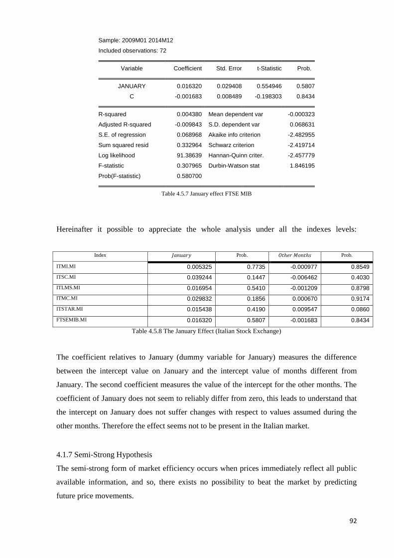
92

Sample: 2009M01 2014M12

Included observations: 72

Variable Coefficient Std. Error t-Statistic Prob.

JANUARY 0.016320 0.029408 0.554946 0.5807

C -0.001683 0.008489 -0.198303 0.8434

R-squared 0.004380 Mean dependent var -0.000323

Adjusted R-squared -0.009843 S.D. dependent var 0.068631

S.E. of regression 0.068968 Akaike info criterion -2.482955

Sum squared resid 0.332964 Schwarz criterion -2.419714

Log likelihood 91.38639 Hannan-Quinn criter. -2.457779

F-statistic 0.307965 Durbin-Watson stat 1.846195

Prob(F-statistic) 0.580700

Table 4.5.7 January effect FTSE MIB

Hereinafter it possible to appreciate the whole analysis under all the indexes levels:

Index 𝐽𝑎𝑛𝑢𝑎𝑟𝑦 Prob. 𝑂𝑡ℎ𝑒𝑟 𝑀𝑜𝑛𝑡ℎ𝑠 Prob.

ITMI.MI 0.005325 0.7735 -0.000977 0.8549

ITSC.MI 0.039244 0.1447 -0.006462 0.4030

ITLMS.MI 0.016954 0.5410 -0.001209 0.8798

ITMC.MI 0.029832 0.1856 0.000670 0.9174

ITSTAR.MI 0.015438 0.4190 0.009547 0.0860

FTSEMIB.MI 0.016320 0.5807 -0.001683 0.8434

Table 4.5.8 The January Effect (Italian Stock Exchange)

The coefficient relatives to January (dummy variable for January) measures the difference

between the intercept value on January and the intercept value of months different from

January. The second coefficient measures the value of the intercept for the other months. The

coefficient of January does not seem to reliably differ from zero, this leads to understand that

the intercept on January does not suffer changes with respect to values assumed during the

other months. Therefore the effect seems not to be present in the Italian market.

4.1.7 Semi-Strong Hypothesis

The semi-strong form of market efficiency occurs when prices immediately reflect all public

available information, and so, there exists no possibility to beat the market by predicting

future price movements.

93

Before assessing the semi-strong efficiency of Italian companies, an example of semi-strong

efficiency is reported in the following rows as an additional explanation of the theory:

Mario Rossi held 100 shares of FCA. He had purchased them on 1 January 2015 for 9,60 €

per share. FCA is a company that appears among the main worldwide car manufacturers.

Mario is not an active investor so he does not checks the stock performance daily. On 12

January 2015 he discovered that FCA has incurred in some trade union troubles by an article

published on 11 January 2012 by Il Sole 24 Ore. According to the article, FCA is wasting

labour time because of an all-out strike. Total outstanding shares of FCA are 1,2 billion.

Mario sold off his holding for 8,5 € per share in the opening hours of 13 January 2012.

Hence, he minimized his loss. Unfortunately, towards the end of 15 January 2015, the

company's stock price had climbed to 10,7 € per share. The market seems to be semi-strong

form efficient because had adjusted itself to the public information on 12 January 2015 as

soon as the market came to know about it and changed on 15 January 2015 when FCA solved

its problems as was shown by a tweet of the FCA CEO Sergio Marchionne.

4.1.1 Methodology

The idea on the basis of this analysis is that if some anomalies affect the Italian market, the

market would result not semi-strong efficient.

The analysis tries to the presence of the Dividend Yield influence over market prices, in order

to study the possibility of the presence of this anomaly and to verify the existence of semi-

strong efficiency into the market.

Dividend Yield

As introduced, another good expedient to keep tracks of stocks behaviours is testing for

dividends. The dividend yield consists in the ratio of the total amount of dividends paid out by

a company in the last year, over the last month. It is possible to analyse the effect of the

dividend yield on some companies on the basis of the following regression:

𝑅𝑡 = 𝜇 + 𝛿′𝐹𝑡−1 + 휀𝑡 (33)

Dividends Yield has been calculated as the ratio between the last dividend paid out and daily

prices. So I constructed a dummy for the month of January and I verified results of the

coefficient.

94

BMPS.MI

Dependent Variable: LOG_RETURNS

Method: Least Squares

Sample: 2/02/2009 1/29/2010

Included observations: 257

Variable Coefficient Std. Error t-Statistic Prob.

DUMDATA4 -0.002624 0.222452 -0.011795 0.9906

C 0.000375 0.062056 0.006049 0.9952

R-squared 0.000001 Mean dependent var 0.000171

Adjusted R-squared -0.003921 S.D. dependent var 0.953477

S.E. of regression 0.955344 Akaike info criterion 2.754261

Sum squared resid 232.7340 Schwarz criterion 2.781880

Log likelihood -351.9226 Hannan-Quinn criter. 2.765368

F-statistic 0.000139 Durbin-Watson stat 2.979286

Prob(F-statistic) 0.990598

Table 4.5.9 Dividend Yield effect BMPS

Results from the regression above suggest that dividend yields do not help investors to

forecast future prices because the coefficient is not really different from zero, as suggested by

a reliable p-value. This means in turn that dividend yields do not appear to influence returns.

R-squared is really low, as confirmed by the F-statistic at 10% significance level. This means

that dividends do not help to explain returns, suggesting that returns are difficult to forecast

and leading not to reject the null hypothesis. Hence the Italian market could be considered

semi-strong form efficient.

The year 2010 was characterized by no dividends for BMPS.

ENI

Dividends Yield has been calculated as the ratio between the total dividend paid out of the

previous year (0,5 + 0,65 for the period 2009) and daily prices.

Dependent Variable: LOG_RETURN

Method: Least Squares

Sample (adjusted): 2/02/2010 1/31/2011

Included observations: 260 after adjustments

95

Variable Coefficient Std. Error t-Statistic Prob.

DIVIDEND_YIELD -0.344979 0.133404 -2.585972 0.0103

C 0.134424 0.051959 2.587088 0.0102

R-squared 0.025265 Mean dependent var 7.63E-05

Adjusted R-squared 0.021487 S.D. dependent var 0.013986

S.E. of regression 0.013835 Akaike info criterion -5.715604

Sum squared resid 0.049381 Schwarz criterion -5.688214

Log likelihood 745.0285 Hannan-Quinn criter. -5.704593

F-statistic 6.687249 Durbin-Watson stat 2.019524

Prob(F-statistic) 0.010259

Table 4.6.0 Dividend Yield effect ENI

Results from the regression above suggest that there exists the possibility that dividend yields

help investors to forecast future prices because the coefficient is different from zero. On the

other hand, the p-value does not suggest considerable reliability results at 5% significance

level. Moreover, neither the F-statistic is considerable significant at 5% statistical level, and

the R-squared and the Adjusted R-squared indicate that the relation between returns and

dividend yields is not considerable. This leads not to reject the null hypothesis, hence the

Italian market could be considered semi-strong form efficient.

Dependent Variable: LOG_RETURN

Method: Least Squares

Sample (adjusted): 2/02/2010 1/31/2011

Included observations: 260 after adjustments

Variable Coefficient Std. Error t-Statistic Prob.

DIVIDEND_YIELD -0.344979 0.133404 -2.585972 0.0103

C 0.134424 0.051959 2.587088 0.0102

R-squared 0.025265 Mean dependent var 7.63E-05

Adjusted R-squared 0.021487 S.D. dependent var 0.013986

S.E. of regression 0.013835 Akaike info criterion -5.715604

Sum squared resid 0.049381 Schwarz criterion -5.688214

Log likelihood 745.0285 Hannan-Quinn criter. -5.704593

F-statistic 6.687249 Durbin-Watson stat 2.019524

Prob(F-statistic) 0.010259

Table 4.6.1 Dividend Yield effect ENI

It is possible to notice the same results for the period from February, 2 2010 to January, 29

2011. The results obtained lead to strongly reject the possibility that dividend yields could

96

help investors to forecast future returns. Hence, ENI seems to be part of a semi-strong

efficient market.

MEDIASET

Dependent Variable: LOG_RETURN

Method: Least Squares

Sample (adjusted): 2/03/2009 1/29/2010

Included observations: 259 after adjustments

Variable Coefficient Std. Error t-Statistic Prob.

DIVIDEND_YIELDS -0.051800 0.040719 -1.272147 0.2045

C 0.015168 0.010690 1.418819 0.1572

R-squared 0.006258 Mean dependent var 0.001654

Adjusted R-squared 0.002391 S.D. dependent var 0.019309

S.E. of regression 0.019285 Akaike info criterion -5.051238

Sum squared resid 0.095586 Schwarz criterion -5.023772

Log likelihood 656.1353 Hannan-Quinn criter. -5.040195

F-statistic 1.618358 Durbin-Watson stat 2.299076

Prob(F-statistic) 0.204471

Table 4.6.2 Dividend Yield effect MS

Dependent Variable: LOG_RETURN

Method: Least Squares

Sample: 2/01/2010 1/31/2011

Included observations: 261

Variable Coefficient Std. Error t-Statistic Prob.

DIVIDEND_YIELD -0.279377 0.190149 -1.469250 0.1430

C 0.026833 0.018692 1.435572 0.1523

R-squared 0.008266 Mean dependent var -0.000575

Adjusted R-squared 0.004437 S.D. dependent var 0.019105

S.E. of regression 0.019063 Akaike info criterion -5.074506

Sum squared resid 0.094120 Schwarz criterion -5.047192

Log likelihood 664.2231 Hannan-Quinn criter. -5.063527

F-statistic 2.158694 Durbin-Watson stat 1.956005

Prob(F-statistic) 0.142979

Table 4.6.3 Dividend Yield effect MS

97

Both in 2009 and 2010, Mediaset issued dividends. Although coefficients differ from zero,

especially in the second case, results do not seem to suggest any affection over returns by

dividends. Indeed R2 and AdjR

2 do not suggest the possibility that this model help finding

relation among returns and dividends.

FINMECCANICA

Dependent Variable: LOG_RETURN

Method: Least Squares

Sample (adjusted): 2/03/2009 1/31/2012

Included observations: 781 after adjustments

Variable Coefficient Std. Error t-Statistic Prob.

DIVIDEND_YIELD -0.029201 0.014072 -2.075073 0.0383

C 0.003806 0.002759 1.379388 0.1682

R-squared 0.005497 Mean dependent var -0.001614

Adjusted R-squared 0.004220 S.D. dependent var 0.024917

S.E. of regression 0.024865 Akaike info criterion -4.548184

Sum squared resid 0.481617 Schwarz criterion -4.536249

Log likelihood 1778.066 Hannan-Quinn criter. -4.543593

F-statistic 4.305928 Durbin-Watson stat 1.899479

Prob(F-statistic) 0.038307

Table 4.6.4 Dividend Yield effect FNC

TELECOM

Dependent Variable: LOG_RETURN

Method: Least Squares

Date: 09/25/15 Time: 11:56

Sample (adjusted): 2/03/2009 1/31/2014

Included observations: 1303 after adjustments

Variable Coefficient Std. Error t-Statistic Prob.

DIVIDEND_YIELD 3.27E-05 0.000135 0.242430 0.8085

C -0.000114 0.000627 -0.182593 0.8551

R-squared 0.000045 Mean dependent var -0.000118

Adjusted R-squared -0.000723 S.D. dependent var 0.022609

S.E. of regression 0.022617 Akaike info criterion -4.738691

Sum squared resid 0.665502 Schwarz criterion -4.730752

Log likelihood 3089.257 Hannan-Quinn criter. -4.735713

98

F-statistic 0.058772 Durbin-Watson stat 2.002185

Prob(F-statistic) 0.808485

Table 4.6.5 Dividend Yield effect TIT

The last two cases examined (Finmeccanica and Telecom) clearly suggest that there exists no

influence carried out by dividends over returns, as confirmed by reliable p-values and despite

the use of larger samples.

5. The ways we access the market

Whomver decides to approach with financial markets would face different opportunities. If

we just think to the Italian Stock Exchange “Borsa Italiana”, there is a wide world of

opportunities. ETFs, ETC, ETM, Mutual Funds, Derivatives, as well as CW, Bonds and

Certificates are the main part of the huge panorama of the Italian Financial Market. Among

these multiple choices of the market, I find interesting to focus on ETFs, which are raising

instruments in the Italian and worldwide panorama.

5.1 Exchange-Traded Funds

Exchange Traded Funds (ETFs) are funds (or Sicav35

) that track indexes like the FTSE MIB,

NASDAQ-100 Index, S&P 500, Dow Jones, etc.36

ETFs are represented as stocks into any

Stock Exchange, that means they are negotiated as a stock as well. ETFs allow to achieve a

yield equal to the benchmark in use. This is possible by means of a passive funds

management style. Another feature of ETFs is represented by the capability to show prices

adjusted for NAV (Net Asset Value)37 38

. ETFs seem to appear as index funds, but they do not

try to outperform their corresponding index, that is a feature of an active management

strategy. Therefore ETFs do not try to beat the market, they try to be the market. As a

consequence, administrative costs of an ETF are supposed to be less than other managed

funds because they incur in less management fees39

.

The origin of ETFs is ascribed to some Canadian instruments (i.e. the Toronto 100 Index

Participation Units - HIPs) by A. Seddik Meziani, but the creator of ETFs is worldwide

35

http://www.borsaitaliana.it/etf/formazione/cosaeunetf/coseunetf.htm 36

http://www.nasdaq.com/investing/etfs/what-are-ETFs.aspx#ixzz3lnDzfJKm 37

The Nav represents the mutual fund’s price per share or the exchange-traded fund’s per share value. The NAV is calculated as the total value of all the securities in its portfolio, divided by the number of fund shares outstanding - http://www.investopedia.com/terms/n/nav.asp 38

http://www.borsaitaliana.it/etf/formazione/cosaeunetf/coseunetf.htm 39

http://www.nasdaq.com/investing/etfs/what-are-ETFs.aspx#ixzz3lnDzfJKm

99

represented by Nathan Most. The first recognized ETF was the Standard & Poor’s Depositary

Receipts (SPDR), also known as “Spider”, based on the S&P500 index. Then, the Barclays

Global Investor fascinated by the success obtained by ETFs in the late 90s, created the World

Equity Benchmark Shares (WEBS), instruments able to replicate any national Stock

Exchange. This leads to the creation of sector ETFs as well 40

. In 2003, the ETF S&P/MIB

Master Unit was born, it was the first ETF over an Italian Stock Exchange index41

. In the

same year, the Active ETF raised up in the NYSE42

, but here the focus is completely

concentred over the traditional concept of ETFs.

ETFs are generally divided in: Management Investment Trust, Unit Investment Trust and

Grantor Trust. Most of the ETFs are structured on the basis of the first typology (MIT, ed.). In

this kind of ETF, managers coordinate activities relative to the underlying. The primary

characteristic of MIT typology is the possibility not to hold each stocks of the underlying (the

index). Unit Investment Trust differs from Management Investment Trust because of the less

flexibility (i.e. no derivatives allowed) and less fees. Finally Grantor Trust is the less

manageable typology, because it is not allowed to hold less stocks than those in the portfolios.

In the Italian Stock Exchange exists a regulated electronic market dedicated to ETFs, the

ETFplus43

. The ETFplus consists of: ETFs, structured ETFs, Active ETFs, Exchange Traded

Commodities (ETC) and Exchange Traded notes (ETN) 44

. It has already been stated the

meaning of ETFs, while structured ETFs add to the normal activity of an ETF, the possibility

to access investment strategies on the basis of a leveraged ETF or a short ETF (this kind of

ETF works on falls of the market). On the other hand ETC and ETN are instruments based on

derivatives and bonds45

. Again, this work is focused just on ETF itself.

5.2 Testing the weak form of EMH through the Exchange-traded Funds in Italy

Given that ETFs represent one of the best ways for an investor to access the market, the last

analysis performed in this work tries to verify the efficiency of the Italian ETFs operating in

the ETFplus market. There exist proofs of the presence of weak form efficiency into the US

40

Strategie basate su indicatori fondamentali e di volatilità: un’applicazione al mercato europeo degli ETF settoriali, Matteo Paolini, 2010 41

Comunicato Stampa, Lyxor AM lancia il primo ETF sull’indice S&P/MIB in Borsa Italiana, 10 Novembre 2003 42

Active ETFs track indexes created by financial managers - Strategie basate su indicatori fondamentali e di volatilità: un’applicazione al mercato europeo degli ETF settoriali, Matteo Paolini, 2010 43

Strategie basate su indicatori fondamentali e di volatilità: un’applicazione al mercato europeo degli ETF settoriali, Matteo Paolini, 2010 44

http://www.borsaitaliana.it/etf/formazione/segmentazioneemicrostrutturamercatoetfplus/etfplussegmentazioneemicrostruttura.htm 45

http://www.borsaitaliana.it/etf/formazione/segmentazioneemicrostrutturamercatoetfplus/etfplussegmentazioneemicrostruttura.htm

100

ETF market46

, this would lead to think there would be in the Italian one as weel. “So, are the

Italian ETFs weak form efficient?” This is the question I would like to answer at the end of

this investigation.

ETFs were born to replicate Index’s performance. The purpose of the management is to make

that total return performance of an ETF trails the total return performance of the benchmark in

order to minimize the differential of the return (Tracking Error)47

. So, the first step in order to

consider whether Italian ETFs are parts of an efficient market, is to evaluate ETFs’

performance with respect to their underlying indexes.

ETFs’ performance has been tested by means of several indicators, Ursula Marchioni of

iShares states that there exist two most important indicators: the tracking difference (TD) and

the aforementioned tracking error (TE)48

.

Tracking Difference

Tracking difference shows how a product’s

performance compares with that of its

benchmark over a significant period of

time49

. Tracking difference results can

appear positive or negative, underlying the

extent to which an ETF outperforms or

underperforms its index. The TD is

computed as the difference between the

NAV (total return) and the total return of the

index (or benchmark). Because the NAV of ETFs total return includes some expenses,

tracking difference typically is negative50

.

Tracking Errors

The first step is to verify how well ETFs track their indexes. In our case Italian ETFs with

available data track all the same index (FTSE MIB). Therefore, following the three estimation

process of the Tracking Error known in literature51

52

, I calculated the TE of four Italian ETFs

46

Testing weak-form e ciency of exchange traded funds market, Gerasimos G. Rompotis, National and Kapodistrian University of Athens, July 2011 47

http://www.borsaitaliana.it/etf/formazione/modalitadireplicaetf/modalitadireplicaetf.htm 48

How to evaluate ETFs through tracking error and difference, Ursula Marchioni. iShares, 2013 49

Understanding tracking difference and tracking error, Vanguard Investments Hong Kong Limited, 2014 50

Understanding tracking difference and tracking error, Vanguard Investments Hong Kong Limited, 2014 51

Tracking S&P 500 index funds. Journal of Portfolio Management, Frino, Gallagher, 2001.

Figure 5.1 How good is your tracker? Use tracking difference

to find out!, The Accumulator, 2011

101

to verify that they follow their indexes at significant level. The tracking errors measure the

difference in performance between the ETF and their benchmark indices53

. In other words,

tracking errors indicate how much variability exists among the individual data points of the

ETF average tracking difference over a given period of time. Therefore, commonly, TE is

defined as the volatility of the differences in returns between an ETF and its underlying index.

Hence, there exist two possibilities: the TE is consistently low, and so, the ETF has been

tracking its underlying index (or benchmark) equally well54

; the TE is not that low, and so it

did not track the ETF consistently.

The three ways to calculate the tracking errors are the following:

The first tracking error is the average of the funds absolute return differences between the

ETF and index, or the mean absolute deviation (MAD):

𝑇𝐸1 =1

𝑇∑ |𝑟𝐹,𝑡 − 𝑟𝑙,𝑡|𝑇

𝑡=1 (34)

The second TE is the standard deviation of return differences between the ETF and the index:

𝑇𝐸2 = √1

𝑇−1∑ (𝑅𝐷𝑇 − 𝑅𝐷̅̅ ̅̅ )2𝑇

𝑡=1 (35)

The last tracking error is calculated as the standard error of a regression of the ETF returns on

the benchmark returns.

𝑇𝐸3 = Standard Error resulted by the following regression:

𝑟𝐹,𝑡 = 𝛼 + 𝛽𝑟𝑙,𝑡 + 𝑢𝑡 (36)

Where 𝑟𝐹,𝑡 and 𝑟𝑙,𝑡 are, respectively, the logarithmic daily return calculated on the NAV of the

ETF considered, and the log daily return of the Index considered. 𝑅𝐷𝑇 it the absolute

52

Measuring the tracking error of exchange traded funds: an unobserved components approach, Giuliano De Rossi, Quantitative analyst, UBS Investment Research, 2012 53

The performance and tracking ability of Exchange Traded Funds, Lars Bassie, Tilburg University – Finance Department, 2012 54

Tracking difference and tracking error of ETFs, Investor Education Centre, Hong Kong

102

difference between 𝑟𝐹,𝑡 and 𝑟𝑙,𝑡. The 𝛽 coefficient of 𝑇𝐸3 measures the co-movement of the

returns of the ETF with the benchmark index. The closer this beta coefficient is to 1, the better

it performs in tracking the index.

The indicator designed to assess Italian ETFs performance is the TE. Following the three

methods and using daily NAV (Net Asset Value) and Daily Log Returns, I computed TEs.

The period of observation fluctuates from October, 22 2010 to September, 9 2015. Results are

the following:

ETF INDEX Tracking

Error

Tracking

Error 2

Tracking

Error 3

AM FT MIB UCITS ETF (FMI.MI) FTSE MIB 0,017804065 0,015602427 0,027962

DBXT FTSE MIB 1D (XMIB.MI) FTSE MIB 0,017196159 0,023187612 0,026852

FTSE MIB EUR (IMIB.MI) FTSE MIB 0,017410839 0,022848089 0,027057

L UC ETF FTS MIB (ETFMIB.MI) FTSE MIB 0,016827193 0,023198928 0,027283

Table 5.1 Tracking Errors over daily ETFs

The table above leads to observe that tracking errors of the selected ETFs fluctuate around a

value 1-3 per cent depending of the estimation process. This leads to think that ETFs well

represent the FTSE MIB index, because the deviation from index values is meaningless

(0,027962 in the worst case). Results state that selected ETFs track FTSE MIB index at a

remarkable level. In other terms, it is possible to affirm that the ETFs performances

correspond to FTSE MIB index. Although the evidences suggest that assesses these ETFs is

unnecessary once that FTSE MIB index has been already tested.

Information Ratio

Another way to assess the efficiency of ETFs, in terms of trailing indexes, is to compute the

Information Ratio (IR).

The IR is an indicator calculated as the ratio between the return differentials and the Tracking

Error.

The formula to calculate the IR is the following:

𝐼𝑅 =𝑅𝑃−𝑅𝐵

𝑇𝐸𝑃,𝐵 (37)

103

Where 𝑅𝑃 is the ETF return, 𝑅𝐵 is the index (or benchmark) return and 𝑇𝐸𝑃,𝐵 is the tracking

error volatility. This indicator includes the weight of return differentials, given the possibility

to check the management capability to outperform the index with respect to the risk (the

contingent gap between ETF and index).

ETF INDEX IR (using

TE)

IR (using

TE 2)

IR (using

TE 3)

AM FT MIB UCITS ETF (FMI.MI) FTSE MIB -4,88165709 -5,570501537 -3,108266282

DBXT FTSE MIB 1D (XMIB.MI) FTSE MIB -1,96499468 -1,457259223 -1,258392697

FTSE MIB EUR (IMIB.MI) FTSE MIB 0,801776152 0,61097432 0,515932877

L UC ETF FTS MIB (ETFMIB.MI) FTSE MIB -0,288829199 -0,2095004 -0,178139676

Table 5.2 Information Ratio over Daily ETFs

The IR adjust for return differential, so it gives a better answer with respect of the TE. Table

5.2 underlines the underperformance of three ETFs, with remarkable evidences for the AM

FT MIB UCITS ETF, while FTSE MIB EUR shows even positive IR values. As a

consequence there exists the possibility that IMIB represents an ETF that outperforms the

market. However values are close to zero, that means ETFs well represent their index. This

does not hold for AM FT MIB UCITS ETF.

Testing the efficiency of ETFs would be an additional useless work on the basis of TE results.

On the other hand, the information ratios suggest the possibility that there exist something

wrong with these ETFs, hence an analysis for the weak-form efficiency have been performed

in the following paragraphs.

5.3 Weak Hypothesis

Purpose of the analysis: An index is a mathematical construct, so it may not be invested in

directly. Exchange-traded funds attempt to track an index in order to transform it into a good

that could be object of investment. The aim of the following analysis is to verify the presence

of weak efficiency into the ETFplus to verify if these instruments are able to give investors a

“cleaning” way to access the market. Therefore the null hypothesis stated is that the prices of

ETFs considered follow a random walk. Hereinafter, the two hypothesis that could be proved:

{𝐻0: 𝑡ℎ𝑒 𝑝𝑟𝑖𝑐𝑒𝑠 𝑜𝑓 𝑡ℎ𝑒 𝐼𝑡𝑎𝑙𝑖𝑎𝑛 𝐸𝑇𝐹𝑠 𝑎𝑟𝑒 𝑟𝑎𝑛𝑑𝑜𝑚 𝑜𝑣𝑒𝑟 𝑡ℎ𝑒 𝑝𝑒𝑟𝑖𝑜𝑑 𝑜𝑓 𝑡ℎ𝑒 𝑠𝑡𝑢𝑑𝑦 − 𝑤𝑒𝑎𝑘 − 𝑓𝑜𝑟𝑚 𝑒𝑓𝑓𝑖𝑐𝑖𝑒𝑛𝑐𝑦

𝐻1: 𝑡ℎ𝑒 𝑝𝑟𝑖𝑐𝑒𝑠 𝑜𝑓 𝑡ℎ𝑒 𝐼𝑡𝑎𝑙𝑖𝑎𝑛 𝐸𝑇𝐹𝑠 𝑎𝑟𝑒 𝑛𝑜𝑡 𝑟𝑎𝑛𝑑𝑜𝑚 𝑜𝑣𝑒𝑟 𝑡ℎ𝑒 𝑝𝑒𝑟𝑖𝑜𝑑 𝑜𝑓 𝑡ℎ𝑒 𝑠𝑡𝑢𝑑𝑦 − 𝑖𝑛𝑒𝑓𝑓𝑖𝑐𝑖𝑒𝑛𝑐𝑦

104

5.4 Data

The analysis relative to the ETFs has been realized by means of Standard Italian ETFs data

obtained by Yahoo finance 55

. There exist seven ETFs belonging to the Italian Stock

Exchange, but I kept out the Lyxor ETF FTSE Italia Mid Cap D-EUR A/I (ITAMID.MI)

because of the small presence of data.

Therefore, ETFs considered are: Amundi FTSE MIB Ucits ETF (FMI.MI), Amundi MSCI

Italy Ucits ETF (CI1.MI), Db X-Trackers FTSE MIB Ucits ETF (Dr) (XMIB.MI), IShares

FTSE MIB Ucits ETF (CSMIB.MI), Lyxor Ucits ETF FTSE MIB (ETFMIB.MI) and

Powershares FTSE Rafi Italy 30 Ucits ETF (PTI.MIB). Even though some of the ETFs’ data

considered are available since 2007, 2008 and 2003, it is not the same for the others.

Therefore, the analysis concerns the period from September, 9 2010 to September, 9 2015.

5.5 Methodology and Results

The analysis follows the guideline of the previous investigations over the Italian market.

Autocorrelation test, ADF and PP tests have been carried out to reach the purpose established

before.

Here an overview of the characteristics of the Italian ETFs selected:

Name Symbol Issuer Benchmark Daily Weekly Monthly

AMUNDI FTSE

MIB UCITS ETF FMI AMUNDI FTSE MIB TR 1224 260 60

AMUNDI MSCI

ITALY UCITS ETF CI1 AMUNDI

MSCI ITALY

TRN 929 240 60

DB X-TRACKERS

FTSE MIB UCITS

ETF (DR)

XMIB DB-X-TRACKERS FTSE MIB 1245 261 60

LYXOR UCITS

ETF FTSE MIB ETFMIB

LYXOR

INTERNATIONAL

ASSET

MANAGEMENT

S.A

FTSE MIB

TRN 1252 261 60

ISHARES FTSE

MIB UCITS ETF

(ACC)

CSMIB ISHARES VII FTSE MIB TR

1186

259 60

POWERSHARES PTI POWERSHARES FTSE RAFI 614 172 60

55

http://www.borsaitaliana.it/etf/etf/home.htm

105

FTSE RAFI ITALY

30 UCITS ETF

GLOBAL FUNDS

IRELAND PLC

ITALY 30

Table 5.3 Profiles of ETFs

Profiles of ETFs underline a lack of available data, not observed before, over Powershares

FTSE RAFI ITALY and AMUNDI MSCI ITALY UCITS ETF. Hereinafter it is possible see

whether this would lead to inconsistent results.

FMI CI1

XMIB ETFMIB

CSMIB PTI

Table 5.4 Time Series Plots of Daily Prices (ETFs)

2.9

3.0

3.1

3.2

3.3

3.4

3.5

3.6

3.7

3.8

IV I II III IV I II III IV I II III IV I II III IV I II III

2011 2012 2013 2014 2015

log price

4.0

4.1

4.2

4.3

4.4

4.5

4.6

4.7

4.8

10 11 12 13 14 15

Log Price

2.5

2.6

2.7

2.8

2.9

3.0

3.1

3.2

3.3

III IV I II III IV I II III IV I II III IV I II III IV I II III

2011 2012 2013 2014 2015

Log Price

2.5

2.6

2.7

2.8

2.9

3.0

3.1

3.2

III IV I II III IV I II III IV I II III IV I II III IV I II III

2011 2012 2013 2014 2015

Log Price

3.6

3.7

3.8

3.9

4.0

4.1

4.2

4.3

4.4

4.5

III IV I II III IV I II III IV I II III IV I II III IV I II III

2011 2012 2013 2014 2015

Log Price

1.0

1.1

1.2

1.3

1.4

1.5

1.6

1.7

1.8

1.9

10 11 12 13 14 15

Log Price

106

FMI CI1

XMIB ETFMIB

CSMIB PTI

Table 5.5 Time Series Plots of Weekly Prices (ETFs)

FMI CI1

3.0

3.1

3.2

3.3

3.4

3.5

3.6

3.7

3.8

III IV I II III IV I II III IV I II III IV I II III IV I II III

2011 2012 2013 2014 2015

Log price

4.0

4.1

4.2

4.3

4.4

4.5

4.6

4.7

4.8

IV I II III IV I II III IV I II III IV I II III IV I II III

2011 2012 2013 2014 2015

Log Price

2.5

2.6

2.7

2.8

2.9

3.0

3.1

3.2

3.3

III IV I II III IV I II III IV I II III IV I II III IV I II III

2011 2012 2013 2014 2015

Log Price

2.5

2.6

2.7

2.8

2.9

3.0

3.1

3.2

III IV I II III IV I II III IV I II III IV I II III IV I II III

2011 2012 2013 2014 2015

Log Price

3.6

3.7

3.8

3.9

4.0

4.1

4.2

4.3

4.4

4.5

III IV I II III IV I II III IV I II III IV I II III IV I II III

2011 2012 2013 2014 2015

Log price

1.0

1.1

1.2

1.3

1.4

1.5

1.6

1.7

1.8

1.9

10 11 12 13 14 15

Log Price

107

XMIB ETFMIB

CSMIB PTI

Table 5.6 Time Series Plots of Monthly Prices (ETFs)

All the plots of ETFs show similar evidences despite the use of different benchmarks. This

would mean that all the benchmark used could reliably represent the underlying portfolio.

FMI CI1

3.0

3.1

3.2

3.3

3.4

3.5

3.6

3.7

3.8

IV I II III IV I II III IV I II III IV I II III IV I II III

2011 2012 2013 2014 2015

Log Price

4.0

4.1

4.2

4.3

4.4

4.5

4.6

4.7

IV I II III IV I II III IV I II III IV I II III IV I II III

2011 2012 2013 2014 2015

Log Price

2.5

2.6

2.7

2.8

2.9

3.0

3.1

3.2

IV I II III IV I II III IV I II III IV I II III IV I II III

2011 2012 2013 2014 2015

Log Price

2.5

2.6

2.7

2.8

2.9

3.0

3.1

3.2

IV I II III IV I II III IV I II III IV I II III IV I II III

2011 2012 2013 2014 2015

Log Price

3.6

3.7

3.8

3.9

4.0

4.1

4.2

4.3

4.4

IV I II III IV I II III IV I II III IV I II III IV I II III

2011 2012 2013 2014 2015

Log price

1.0

1.1

1.2

1.3

1.4

1.5

1.6

1.7

1.8

1.9

IV I II III IV I II III IV I II III IV I II III IV I II III

2011 2012 2013 2014 2015

Log Price

108

XMIB ETFMIB

CSMIB PTI

Table 5.7 Time Series Plots of Daily Log Returns (ETFs)

FMI CI1

-.08

-.06

-.04

-.02

.00

.02

.04

.06

.08

IV I II III IV I II III IV I II III IV I II III IV I II III

2011 2012 2013 2014 2015

log return

-.12

-.08

-.04

.00

.04

.08

.12

10 11 12 13 14 15

Log Return

-.08

-.06

-.04

-.02

.00

.02

.04

.06

.08

III IV I II III IV I II III IV I II III IV I II III IV I II III

2011 2012 2013 2014 2015

Log Return

-.08

-.06

-.04

-.02

.00

.02

.04

.06

.08

III IV I II III IV I II III IV I II III IV I II III IV I II III

2011 2012 2013 2014 2015

Log Return

-.12

-.08

-.04

.00

.04

.08

III IV I II III IV I II III IV I II III IV I II III IV I II III

2011 2012 2013 2014 2015

Log Return

-.15

-.10

-.05

.00

.05

.10

.15

10 11 12 13 14 15

Log Return

109

XMIB ETFMIB

CSMIB PTI

Table 5.8 Time Series Plots of Weekly Log Returns (ETFs)

FMI CI1

-.15

-.10

-.05

.00

.05

.10

.15

III IV I II III IV I II III IV I II III IV I II III IV I II III

2011 2012 2013 2014 2015

log return

-.15

-.10

-.05

.00

.05

.10

.15

IV I II III IV I II III IV I II III IV I II III IV I II III

2011 2012 2013 2014 2015

Log Return

-.15

-.10

-.05

.00

.05

.10

.15

III IV I II III IV I II III IV I II III IV I II III IV I II III

2011 2012 2013 2014 2015

Log Return

-.15

-.10

-.05

.00

.05

.10

.15

III IV I II III IV I II III IV I II III IV I II III IV I II III

2011 2012 2013 2014 2015

Log Return

-.15

-.10

-.05

.00

.05

.10

III IV I II III IV I II III IV I II III IV I II III IV I II III

2011 2012 2013 2014 2015

Log Return

-.20

-.15

-.10

-.05

.00

.05

.10

.15

10 11 12 13 14 15

Log Return

110

XMIB ETFMIB

CSMIB PTI

Table 5.9 Time Series Plots of Monthly Log Returns (ETFs)

As expected, Log Returns plots show high volatility of data.

Daily analysis

Descriptive Analysis

Symbol Mean Median St.Dev. Min Max Kurtosis Skewness

FMI 30.10387 30.65750 5.382371 19.87270 41.45000 2.041567 0.148740

CI1 82.86021 84.52000 13.79790 56.78600 111.1200 1.946983 0.057908

XMIB 18.89311 19.22500 3.075260 12.49400 24.62000 1.724829 -0.026387

-.20

-.15

-.10

-.05

.00

.05

.10

.15

IV I II III IV I II III IV I II III IV I II III IV I II III

2011 2012 2013 2014 2015

Log Return

-.20

-.15

-.10

-.05

.00

.05

.10

.15

IV I II III IV I II III IV I II III IV I II III IV I II III

2011 2012 2013 2014 2015

Log Return

-.20

-.16

-.12

-.08

-.04

.00

.04

.08

.12

IV I II III IV I II III IV I II III IV I II III IV I II III

2011 2012 2013 2014 2015

Log Return

-.20

-.16

-.12

-.08

-.04

.00

.04

.08

.12

IV I II III IV I II III IV I II III IV I II III IV I II III

2011 2012 2013 2014 2015

Log Return

-.20

-.16

-.12

-.08

-.04

.00

.04

.08

.12

IV I II III IV I II III IV I II III IV I II III IV I II III

2011 2012 2013 2014 2015

Log Return

-.20

-.15

-.10

-.05

.00

.05

.10

.15

IV I II III IV I II III IV I II III IV I II III IV I II III

2011 2012 2013 2014 2015

Log Return

111

ETFMIB 18.69343 19.02950 2.968080 12.42000 24.17400 1.749224 -0.060236

CSMIB 59.65849 60.76500 10.66936 39.47270 81.98000 2.033558 0.169626

PTI 4.955149 5.205650 0.825061 2.896000 6.220000 2.469477 -0.695217

Table 5.1.0 Daily Descriptive Analysis (ETFs)

Unit Root test

In order to apply the analysis for unit roots, it has been used log prices.

Augmented Dickey-Fuller Test

The ADF test comes again to help assessing the existence of a unit root in the log prices time

series of the six Italian ETFs, or to assess whether the price series are stationary or not. The

second case represents inefficiency. These unit root test are carried out with a constant.

The hypothesis that ETFs’ prices follow a RW would prove the weak efficiency. The idea is

to verify the null hypothesis of the presence of a unit root:

Hence,

{𝐻0: 𝜑 = 1

𝐻1: |𝜑| < 1

under the null hypothesis 𝑥𝑡~𝐼(1), while the alternative is represented by an autoregressive

stationary process (𝑥𝑡~𝐼(0)).

LEVEL

FMI CI1 XMIB ETFMIB CSMIB PTI

t-Statistic -1.249632 -1.409246 -1.539639 -1.661770 -1.257970 -1.446427

Prob.* 0.6546 0.5789 0.5133 0.4506 0.6508 0.5602

TEST CRITICAL VALUE

1% level -3.435484 -3.437175 -3.435394 -3.435365 -3.435654 -3.440788

5% level -2.863695 -2.864442 -2.863655 -2.863642 -2.863770 -2.866037

10% level -2.567967 -2.568368 -2.567946 -2.567939 -2.568008 -2.569223

*MacKinnon (1996) one-sided p-values.

Table 5.1.1 ADF Test for Daily log prices - ETFs (level)

All the results of the ETFs underline values smaller than the critical ones. This means that all

the ETFs show the presence of a unit root, so the null hypothesis cannot be rejected. P-values

confirm results at all significance levels. Hence, it is possible to affirm that the market has

been proved to be weak form efficient.

112

Philip-Perron Test

LEVEL

FMI CI1 XMIB ETFMIB CSMIB PTI

t-Statistic -1.174297 -1.275307 -1.499431 -1.613559 -1.136033 -1.497694

Prob.* 0.6875 0.6428 0.5338 0.4753 0.7034 0.5343

TEST CRITICAL VALUE

1% level -3.435484 -3.437175 -3.435394 -3.435365 -3.435654 -3.440788

5% level -2.863695 -2.864442 -2.863655 -2.863642 -2.863770 -2.866037

10% level -2.567967 -2.568368 -2.567946 -2.567939 -2.568008 -2.569223

*MacKinnon (1996) one-sided p-values.

Table 5.1.2 PP Test for Daily log prices - ETFs (level)

The PP test, examining the long run effects into the short run dynamic by means of long run

variance, confirm the ADF conclusions. Indeed, all the ETFs considered appear to have a unit

root, and all p-values affirm that results are significant at 1%, 5% and 10% level.

Serial Correlation Test

{

𝐻0: 𝐷𝑎𝑡𝑎 𝑎𝑟𝑒 𝑖𝑛𝑑𝑒𝑝𝑒𝑛𝑑𝑒𝑛𝑡𝑙𝑦 𝑑𝑖𝑠𝑡𝑟𝑖𝑏𝑢𝑡𝑒𝑑 (𝑡ℎ𝑒 𝑐𝑜𝑟𝑟𝑒𝑙𝑎𝑡𝑖𝑜𝑛𝑠 𝑎𝑟𝑒 𝑒𝑞𝑢𝑎𝑙 𝑡𝑜 𝑧𝑒𝑟𝑜, 𝑠𝑜 𝑎𝑛𝑦 𝑜𝑏𝑠𝑒𝑟𝑣𝑒𝑑 𝑐𝑜𝑟𝑟𝑒𝑙𝑎𝑡𝑖𝑜𝑛𝑠 𝑟𝑒𝑠𝑖𝑙𝑡 𝑓𝑟𝑜𝑚 𝑟𝑎𝑛𝑑𝑜𝑚𝑛𝑒𝑠𝑠)

𝐻1: 𝑇ℎ𝑒 𝑑𝑎𝑡𝑎 𝑎𝑟𝑒 𝑛𝑜𝑡 𝑖𝑛𝑑𝑒𝑝𝑒𝑛𝑑𝑒𝑛𝑡𝑙𝑦 𝑑𝑖𝑠𝑡𝑟𝑖𝑏𝑢𝑡𝑒𝑑 (𝑠𝑒𝑟𝑖𝑎𝑙 𝑐𝑜𝑟𝑟𝑒𝑙𝑎𝑡𝑖𝑜𝑛)

FMI CI1

113

XMIB ETFMIB

CSMIB PTI

114

Table 5.1.3 Serial Correlation of Daily log prices - ETFs

Even for ETFs, results show tendency to be equal to zero, with reliable p-values over many

lags. This leads not to reject the null hypothesis, so the weak form efficiency could be

confirmed.

Weekly analysis

Descriptive Analysis

Symbol Average Median St.Dev. Min Max Kurtosis Skewness

FMI 30.21355 30.86250 5.375319 20.21000 41.08000 2.036904 0.122903

CI1 82.75414 82.75414 13.74313 57.58000 109.8900 1.951775 0.132985

XMIB 18.93727 19.29000 3.079632 13.11500 24.45500 1.729187 -0.043066

ETFMIB 18.73949 19.08000 2.972988 12.95300 24.17400 1.751527 -0.074414

CSMIB 59.94001 61.22000 10.60562 40.13000 81.42000 2.028026 0.119471

PTI 4.839880 5.092700 0.891918 2.925300 6.205000 2.078797 -0.508082

Table 5.1.4 Descriptive Analysis of Weekly log prices - ETFs

Unit Root test

Augmented Dickey-Fuller Test

115

LEVEL

FMI CI1 XMIB ETFMIB CSMIB PTI

t-Statistic -1.137939 -1.341879 -1.444952 -1.581016 -1.140459 -1.277937

Prob.* 0.7012 0.6102 0.5600 0.4909 0.7001 0.6394

TEST CRITICAL VALUE

1% level -3.455486 -3.457630 -3.455387 -3.455387 -3.455585 -3.468749

5% level -2.872499 -2.873440 -2.872455 -2.872455 -2.872542 -2.878311

10% level -2.572684 -2.573187 -2.572660 -2.572660 -2.572707 -2.575791

*MacKinnon (1996) one-sided p-values.

Table 5.1.5 ADF Test for Weekly log prices - ETFs (level)

The weekly log prices give back same results as before, strongly confirming the null

hypothesis at all significance levels. It is possible to see that high significant p-values confirm

results both for the above ADF test that for the below PP test as well.

Philip-Perron Test

LEVEL

FMI CI1 XMIB ETFMIB CSMIB PTI

t-Statistic -1.142268 -1.258622 -1.512727 -1.593731 -1.160811 -1.337988

Prob.* 0.6994 0.6490 0.5258 0.4843 0.6917 0.6113

TEST CRITICAL VALUE

1% level -3.455486 -3.457630 -3.455387 -3.455387 -3.455585 -3.468749

5% level -2.872499 -2.873440 -2.872455 -2.872455 -2.872542 -2.878311

10% level -2.572684 -2.573187 -2.572660 -2.572660 -2.572707 -2.575791

*MacKinnon (1996) one-sided p-values.

Table 5.1.6 PP Test for Weekly log prices - ETFs (level)

Serial Correlation Test

{

𝐻0: 𝐷𝑎𝑡𝑎 𝑎𝑟𝑒 𝑖𝑛𝑑𝑒𝑝𝑒𝑛𝑑𝑒𝑛𝑡𝑙𝑦 𝑑𝑖𝑠𝑡𝑟𝑖𝑏𝑢𝑡𝑒𝑑 (𝑡ℎ𝑒 𝑐𝑜𝑟𝑟𝑒𝑙𝑎𝑡𝑖𝑜𝑛𝑠 𝑎𝑟𝑒 𝑒𝑞𝑢𝑎𝑙 𝑡𝑜 𝑧𝑒𝑟𝑜, 𝑠𝑜 𝑎𝑛𝑦 𝑜𝑏𝑠𝑒𝑟𝑣𝑒𝑑 𝑐𝑜𝑟𝑟𝑒𝑙𝑎𝑡𝑖𝑜𝑛𝑠 𝑟𝑒𝑠𝑖𝑙𝑡 𝑓𝑟𝑜𝑚 𝑟𝑎𝑛𝑑𝑜𝑚𝑛𝑒𝑠𝑠)

𝐻1: 𝑇ℎ𝑒 𝑑𝑎𝑡𝑎 𝑎𝑟𝑒 𝑛𝑜𝑡 𝑖𝑛𝑑𝑒𝑝𝑒𝑛𝑑𝑒𝑛𝑡𝑙𝑦 𝑑𝑖𝑠𝑡𝑟𝑖𝑏𝑢𝑡𝑒𝑑 (𝑠𝑒𝑟𝑖𝑎𝑙 𝑐𝑜𝑟𝑟𝑒𝑙𝑎𝑡𝑖𝑜𝑛)

FMI CI1

116

XMIB ETFMIB

CSMIB PTI

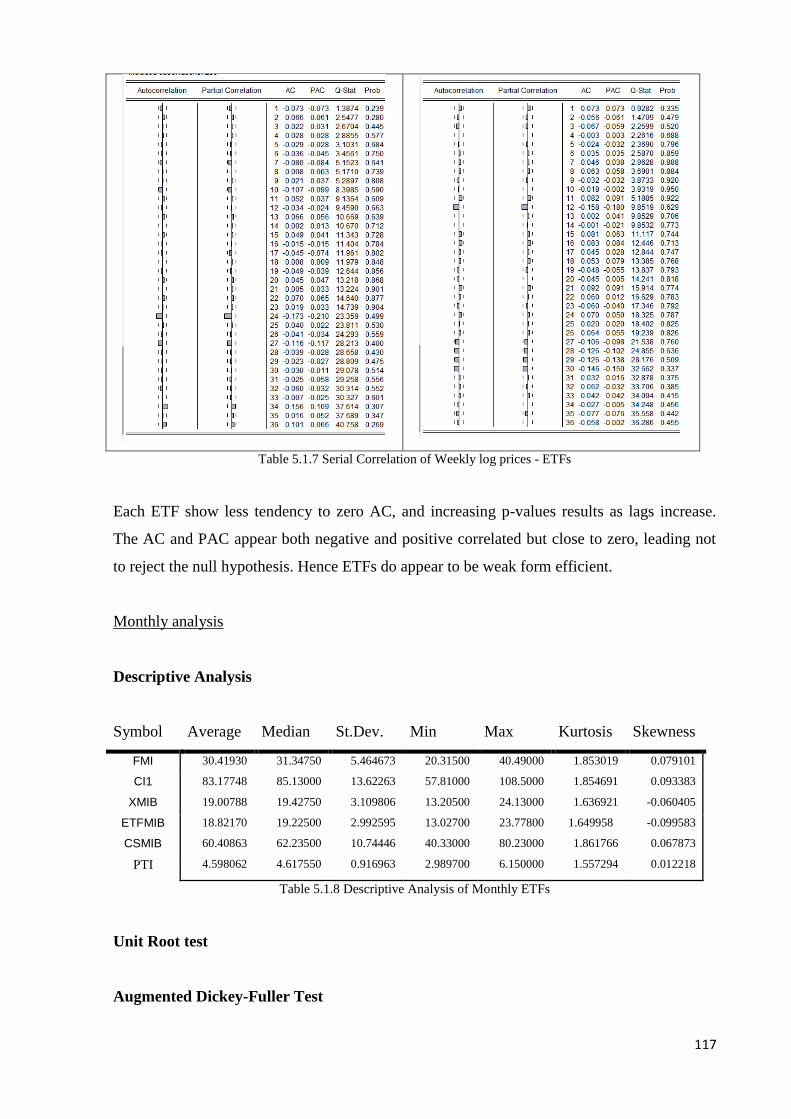
117

Table 5.1.7 Serial Correlation of Weekly log prices - ETFs

Each ETF show less tendency to zero AC, and increasing p-values results as lags increase.

The AC and PAC appear both negative and positive correlated but close to zero, leading not

to reject the null hypothesis. Hence ETFs do appear to be weak form efficient.

Monthly analysis

Descriptive Analysis

Symbol Average Median St.Dev. Min Max Kurtosis Skewness

FMI 30.41930 31.34750 5.464673 20.31500 40.49000 1.853019 0.079101

CI1 83.17748 85.13000 13.62263 57.81000 108.5000 1.854691 0.093383

XMIB 19.00788 19.42750 3.109806 13.20500 24.13000 1.636921 -0.060405

ETFMIB 18.82170 19.22500 2.992595 13.02700 23.77800 1.649958 -0.099583

CSMIB 60.40863 62.23500 10.74446 40.33000 80.23000 1.861766 0.067873

PTI 4.598062 4.617550 0.916963 2.989700 6.150000 1.557294 0.012218

Table 5.1.8 Descriptive Analysis of Monthly ETFs

Unit Root test

Augmented Dickey-Fuller Test

118

LEVEL

FMI CI1 XMIB ETFMIB CSMIB PTI

t-Statistic -0.946420 -1.147735 -1.320984 -1.418300 -1.011838 -1.207373

Prob.* 0.7664 0.6910 0.6142 0.5674 0.7436 0.6657

TEST CRITICAL VALUE

1% level -3.546099 -3.546099 -3.546099 -3.546099 -3.546099 -3.546099

5% level -2.911730 -2.911730 -2.911730 -2.911730 -2.911730 -2.911730

10% level -2.593551 -2.593551 -2.593551 -2.593551 -2.593551 -2.593551

*MacKinnon (1996) one-sided p-values.

Table 5.1.9 ADF Test for Monthly log prices - ETFs (level)

ADF test over Monthly log prices of the selected ETFs show, again, the impossibility to reject

the null hypothesis. Results appear really strong especially for the FMI.MI, that shows a

statistic value of -0.946420, on the basis of a p-value of 0.7664.

Philip-Perron Test

LEVEL

FMI CI1 XMIB ETFMIB CSMIB PTI

t-Statistic -1.033526 -1.147735 -1.425537 -1.524286 -1.075665 -1.207373

Prob.* 0.7357 0.6910 0.5638 0.5145 0.7198 0.6657

TEST CRITICAL VALUE

1% level -3.546099 -3.546099 -3.546099 -3.546099 -3.546099 -3.546099

5% level -2.911730 -2.911730 -2.911730 -2.911730 -2.911730 -2.911730

10% level -2.593551 -2.593551 -2.593551 -2.593551 -2.593551 -2.593551

*MacKinnon (1996) one-sided p-values.

Table 5.2.0 PP Test for Monthly log prices - ETFs (level)

Here, as before in the ADF test, results show the possibility to be able to approve the weak

efficicency of the ETFs considered.

Serial Correlation Test

{

𝐻0: 𝐷𝑎𝑡𝑎 𝑎𝑟𝑒 𝑖𝑛𝑑𝑒𝑝𝑒𝑛𝑑𝑒𝑛𝑡𝑙𝑦 𝑑𝑖𝑠𝑡𝑟𝑖𝑏𝑢𝑡𝑒𝑑 (𝑡ℎ𝑒 𝑐𝑜𝑟𝑟𝑒𝑙𝑎𝑡𝑖𝑜𝑛𝑠 𝑎𝑟𝑒 𝑒𝑞𝑢𝑎𝑙 𝑡𝑜 𝑧𝑒𝑟𝑜, 𝑠𝑜 𝑎𝑛𝑦 𝑜𝑏𝑠𝑒𝑟𝑣𝑒𝑑 𝑐𝑜𝑟𝑟𝑒𝑙𝑎𝑡𝑖𝑜𝑛𝑠 𝑟𝑒𝑠𝑖𝑙𝑡 𝑓𝑟𝑜𝑚 𝑟𝑎𝑛𝑑𝑜𝑚𝑛𝑒𝑠𝑠)

𝐻1: 𝑇ℎ𝑒 𝑑𝑎𝑡𝑎 𝑎𝑟𝑒 𝑛𝑜𝑡 𝑖𝑛𝑑𝑒𝑝𝑒𝑛𝑑𝑒𝑛𝑡𝑙𝑦 𝑑𝑖𝑠𝑡𝑟𝑖𝑏𝑢𝑡𝑒𝑑 (𝑠𝑒𝑟𝑖𝑎𝑙 𝑐𝑜𝑟𝑟𝑒𝑙𝑎𝑡𝑖𝑜𝑛)

119

FMI CI1

XMIB ETFMIB

CSMIB PTI

120

Table 5.2.1 Serial Correlation of Monthly log prices - ETFs

Each ETF, analysed on the basis of Monthly data, show less tendency to zero AC, and

increasing p-values results as lags increase. The AC and PAC appear both negative and

positive correlated, leading not to reject the null hypothesis. Again, ETFs do appear to be

weak form efficient.

121

Conclusions

The analysis carried out has shown some significance relative to the efficiency of the Italian

market. Although there exist proofs of the weak efficiency of the market, few indexes and

companies rejected the random walk hypothesis. This leads not to completely confirm the

efficiency of the market. The analysis for the semi-strong form has been computed observing

the dividend yields impact over returns, showing absence of any influence by dividends

announcement (or issues). Hence, it is possible to think at the Italian market as a weak and

semi-strong form efficient market. Therefore, as underlined by a long literature, the efficient

market hypothesis has been strongly challenged. A part from the evidences emerged by

econometrics analysis, that can, or cannot, be proved nowadays, one of the big deal that the

EMH has to face. is represented by renowned traders that are in contact with many investors

whose ask for advice. I take my personal experience as an example. During a seminar at

Giotto SIM in Padua, I listened the trader Giovanni Borsi explaining easily this concept:

movements of masses represent a profitable information that some traders could get in

advance because investors literally told them what they are going to do. This could represent

an information that the trader himself obtains to beat the market. Moreover Borsi, actually

focused on Banca Monte dei Paschi di Siena issue, explained that he usually speaks with

some professionals of the Bank with whom he compares his forecasting thoughts about future

trends over the BMPS.MI. Beyond the fact that during all the seminar I could not avoid to

think that Borsi was just showing his skills to scrape together clients, I want to make some

considerations on his speech. Indeed, even if a single, or a few groups of traders, really got

some information in advice with respect to the market, this would not mean that they are able

to exploit them. The investors that ask them for advice would make their own finally move,

more or less linked to rational or irrational thoughts. There exist no possibility that all

investors gathered could outperform in turn the market on the basis of a well-known

anomalies of the market. Borsi himself underlined that investors try to exploit the January

effect yet. The consequence is just that everyone tries to buy or sell at the same time, so none

becomes able to beat the market. However Borsi stated that knowing these attitude of

investors, he beat the market with a move in advance based on investors’ information. The

problem is that if all traders with “information in advance” think to the same moves, hence

there is no information to exploit, they will generate the same flow in the market. Clearly the

confuse and twisted speech underlined could be interpreted as a chess game in which

investors should know at least three or four moves to do in advice with respect to the market.

The existence in past of certain anomalies could not be deny, but as the same Borsi explained,

nowadays practically feasibility shows that investors do not be able to exploit them to beat the

122

market. That means the investors themselves, as part of the market, canceled the anomalies.

This could lead to agree with Andrew Lo’s theory of an Adaptive Market56

in which the

efficiency of the market depends on the environment. However the Adaptive Market theory is

none other than an extension of the efficient market hypothesis. Again, Borsi stated that,

basically, him could not periodically gain from the market just by carrying out some

strategies. He affirmed that this game would be effective just when it is played at full time,

but I imagine investors would join at least the seven or eight sleeping hours. A part from

jokes, maybe the real potshots of the EMH are represented by financial crisis. In fact an

efficient market is supposed to include all the available public information (semi-strong

efficiency). The problem occurs when public information do not reflect the real situation of a

market because of forgery or other issues. However my opinion is that these kind of troubles

are characteristic of a strong form of efficiency, that is not object of the current debate.

After this parenthesis is useful to go back on the current results, aware of the fact that there

exist other approaches to assess the EMH, but the econometrics one is the approach assumed

to be more reliable under my point of view. As asserted by Edwards Deming, what count are

data.

Results obtained suggest that not all the component owned by the Italian Stock Exchange

respect the random walk hypothesis, few analysis revealed the presence of serial correlation

among prices rather than the absence of unit roots as a proof of the non-efficiency. If we look

just at the specific case of the ETFplus market, results suggests a good degree of weak form

efficiency on the basis of the represented Italian ETFs.

Many time the truth is somewhere in-between. So, is it possible that the market is efficient but

some exogenous events can briefly affect the market leaving it to remain efficient? In other

words, is it possible that the inefficiency of the market is so temporary that could not be

classified as inefficiency?

My conclusion will not be somewhere in-between. Considering the whole analysis performed

the Italian Market results at least weak form efficient. The possibility to outperform the

market do not appear so evident to classified the market out of the first two forms defined by

Fama. Obviously the present analysis is a drop in the bucket compared with the whole

literature generated by the EMH, but it represents a recent proof of the fact that the

complexity of any market, especially the Italian one, could not be so easily interpreted. To

approach with financial markets means to be aware of the possibility to face markets with a

variety of treats and non-physical walls that an inexpert investors could suffer. Beyond the

56

A theory developed in 2004 by Andrew Lo (MIT) that tries to gather the efficient market hypothesis to the behavioral finance.

123

trading possibility the market was born to exchange financial instruments and support

companies in which someone trust. The starting point to approach any market is to know it.

The weak form efficiency of the Italian market, and the awareness that it includes some

potshots, supplies the basic knowledge that anyone need to be a conscious investor, or

analyst, or any other financial professional going near this interesting field.

124

References:

- History of the Efficient Market Hypothesis, Martin Sewell, 2011, UCL Department of

Computer Science

- On Modelling Speculative Prices: The Empirical Literature, Elena Andreou, Nikitas Pittis,

Aris Spanos

- A Random Walk Down Wall Street, Burton G. Malkiel

- The Econometrics of Financial Markets, John Y. Campbell, Andrew W. Lo, A. Craig

MacKinlay, Princeton University Press, 1997

- The Efficient Market Hypothesis and Its Critics, Burton G. Malkiel, Princeton University,

CEPS Working Paper No. 91, 2003

- From Efficient Market Hypothesis to Behavioural Finance: Can Behavioural Finance be the

new dominant model for investing?, A. Konstantinidis, A. Katarachia, G. Borovas, M. E.

Voutsa, Scientific Bulletin – Economic Sciences, Vol. 11/Issue 2

- Dispensa di Econometria delle Serie Storiche, Giulio Palomba, 2014

- http://www.itl.nist.gov/div898/handbook/eda/section3/eda35d.htm

- Trend e Radici Unitarie, Matteo Pelagatti, 2007

- Analisi Econometrica delle serie storiche con R, Sergio Salvino Guirreri, Università degli

studi di Palermo, Dipartimento di Scienze Statistiche e Matematiche “S. Vianelli”, Dottorato

di Ricerca in Statistica e Finanza Quantitativa – XXI Ciclo

- Il Mercato Azionario, Franco Caparrelli, 1995

- The Semi-Strong Efficiency Debate: in Search of a New Testing Framework, Arianna Ziliotto,

Massimiliano Serati, Carlo Cattaneo LIUC University School of Economics and

Management, February 2015

- Market Efficiency, Market Anomalies, Causes, Evidences, and Some Behavioral Aspects of

Market Anomalies, M. Latif, S. Arshad, M. Fatima, S. Farooq, Institute of Management

Sciences Bahauddin Zakaria University, Multan, Pakistan, 2011

- Anomalies and Market Efficiency. G. William Schwert, University of Rochster, and NBER,

2003

- Calendar-effects.behaviouralfinance.net/

- Il Mercato Azionario Italiano: efficienza e anomalie di calendario, E. Barone, 1990

- http://www.performancetrading.it/Documents/MpMercati/MpM_cAnomalie.htm

- Testing the Efficient Market Hypothesis and its Critics – Application on the Montenegrin

Stock Exchange, Tamara Backovic Vulic, MSc University of Montenegro, Podgorica Faculty

125

of Economics, professor assistant of Econometrics, Business Statistics, Operations Research,

Applied Econometrics and Decision Making Models

- http://thismatter.com/money/investments/market-anomalies.htm

- Finanza Aziendale 2, Roberta Pace, 2009

- The neglected firm effect and an application in Istanbul Stock Exchange, Soner Akkoc,

Mustafa Mesut Kayali, Metin Ulukoy, Banks and Bank Systems, Volume 4, Issue 3, 2009

- The Size Effect, Brian T. Brian T. Allman et al, 2009

- http://stockcharts.com/school/doku.php?id=chart_school:overview:fundamental_analysis

- http://www.investorhome.com/anomtec.htm

- Anomalie di calendario: l'effetto ora legale, Boido, Claudio, Fasano, Antonio, Periodico: AF.

Analisi finanziaria, 2004

- Econometria, Volume 1, Franco Angeli

- Econometria Applicata – Un’introduzione, Massimiliano Marcellino

- Introduzione all’Econometria. Nunzio Cappuccio, Renzo Orsi

- Risk and the January Effect in the Market for the US Dollar, R.S. Rathinasamy, Krishna G.

Mantripragada, Charmen Loh

- Introduzione alla statistica non parametrica, Luigi Salmaso

- Elementi di Statistica Descrittiva per distribuzioni univariate, Metodi non parametrici per un

campione, Maria Pia D’Ambrosio, Franco Anzani, Six Sigma

- Introduzione all’Econometria, N.Cappuccio, R.Orsi

- Strategie basate su indicatori fondamentali e di volatilità: un’applicazione al mercato

europeo degli ETF settoriali, Matteo Paolini, Università degli studi di Modena e Reggio

Emilia “Marco Biagi”, 2010

- www.borsaitaliana.it

- Testing weak-form e ciency of exchange traded funds market, Gerasimos G. Rompotis,

National and Kapodistrian University of Athens, July 2011

- Measuring the tracking error of exchange traded funds: an unobserved components

approach, Giuliano De Rossi, Quantitative analyst, UBS Investment Research, 2012

- Tracking S&P 500 index funds. Journal of Portfolio Management, Frino A., Gallagher D.,

2001

- The performance and tracking ability of Exchange Traded Funds, Lars Bassie, Tilburg

University – Finance Department, 2012

- How to evaluate ETFs through tracking error and difference, Ursula Marchioni. iShares,

2013

- Tracking difference and tracking error of ETFs, Investor Education Centre, Hong Kong