
Automatic chord recognition using Deep Learning techniques · POLITECNICO DI MILANO acoltàF di...
120
-
Upload
nguyenngoc -
Category
Documents
-
view
226 -
download
0
Transcript of Automatic chord recognition using Deep Learning techniques · POLITECNICO DI MILANO acoltàF di...

POLITECNICO DI MILANO
Facoltà di Ingegneria dell'Informazione
Corso di Laurea Magistrale in Ingegneria e Design del suono
Dipartimento di Elettronica e Informazione
Automatic chord recognition using Deep
Learning techniques
Supervisor: Prof. Augusto Sarti
Assistant supervisor: Dr. Massimiliano Zanoni
Master graduation thesis by:
Alessandro Bonvini, ID 783837
Academic Year 2012-2013

POLITECNICO DI MILANO
Facoltà di Ingegneria dell'Informazione
Corso di Laurea Magistrale in Ingegneria e Design del suono
Dipartimento di Elettronica e Informazione
Riconoscimento automatico di accordi
usando tecniche di Deep Learning
Relatore: Prof. Augusto Sarti
Correlatore: Dr. Massimiliano Zanoni
Tesi di Laurea Magistrale di:
Alessandro Bonvini, ID 783837
Anno Accademico 2012-2013


Abstract
The past few years have been characterized by the growing availability of
multimedia content that, nowadays, can be easily retrieved, shared and mod-
ied by people in every corner of the world.
Music has been strongly involved in this innovation and, thanks to the
advent of digital audio format, has become one of the most investigated
elds. This brought to the born of a branch of Information Retrieval that
specically deals on capturing useful information from musical content called
Music Information Retrieval (MIR).
One of the main eorts of MIR researchers in the last period has been to
create methods to automatically extract meaningful descriptors from audio
les. The chord transcription belongs to this category and it can be used as
input feature by other MIR systems.
Having a good chord transcription of a song is becoming an increasing
need for musicians. Ocial transcription are dicult to nd in the Internet
since they are not always published and in many cases are hand-made by
not professional musicians.
The rst step of the automatic chord recognition (ACR) is the extraction
of a meaningful descriptor that enhances the contribution of every note at
each instant. One of the main strategies of doing ACR is based on the com-
parison of vectors of the extracted descriptor with a set of chords templates
by means of a distance measure. This method, due to the interaction of
many instruments with dierent timbral characteristics, is very inuenced
by the noise of the descriptor itself and, for this reason, can be ineective.
In this work we propose a method for Automatic Chord Recognition based
on machine learning techniques. These techniques are designed to auto-
matically learn the complicated relations that link an input observation to
the corresponding class making use of probabilistic theory. In this work,
we tested the accuracy of linear and non linear classiers and the recent
Deep Learning techniques showing that they can be a good alternative to
the template-matching based methods for ACR.
I


Sommario
Gli ultimi anni sono stati caratterizzati da una crescente disponibilità di con-
tenuto multimediale che, ai giorni nostri, può essere facilmente recuperato,
condiviso e modicato da persone in ogni angolo del mondo.
La musica è stata fortemente coinvolta in questa innovazione e, grazie
all'avvento del formato audio digitale, è diventata uno dei campi più investi-
gati. Questo ha portato, negli ultimi anni, alla nascita di una nuova branca
dell'Information Retrieval che si occupa specicamente di catturare infor-
mazioni utili da contenuto musicale chiamata Music Information Retrieval
(MIR).
Uno dei principali sforzi dei ricercatori di MIR nell'ultimo periodo è stato
di creare metodi per estrarre automaticamente descrittori signicativi dai
le audio. La trascrizione di accordi rientra in questa categoria e puo essere
a sua volta utilizzata come descrittore da altri sistemi di MIR.
Avere una buona trascrizione di accordi, inoltre, sta diventando una ne-
cessitá crescente per i musicisti. Trascrizioni uciali sono dicili da trovare
in Internet in quanto non sono sempre pubblicate e in molti casi sono fatte
a mano da musicisti non professionisti. La trascrizione di accordi può anche
essere usata come descrittore in ingresso ad altri sistemi MIR.
Il primo passo della trascrizione automatica di accordi (TAA) è l'estrazione
di un descrittore informativo che metta in evidenza il contributo di ogni nota
in ogni istante. Una delle principali strategie nel fare riconoscimento auto-
matico di accordi, è basata sul confronto tra vettori del descrittore estratto
con un insieme di templates di accordi attraverso una misura di distanza.
Questo metodo, a causa dell'interazione tra tanti strumenti con diverse carat-
teristiche timbriche, è molto inuenzato dal rumore del descrittore stesso
e, per questa ragione, puó essere inecace. In questa tesi proponiamo un
metodo per fare TAA basato su tecniche di machine learning. Queste tec-
niche sono progettate per imparare automaticamente le complicate relazioni
che legano un'osservazione alla corrispondente classe facendo uso della teoria
probabilistica. In questo lavoro abbiamo testato l'accuratezza di classica-
III

tori lineari e non lineari e le recenti tecniche di Deep Learning, mostrando che
possono essere una buona alternativa ai metodi di confronto tra templates
per quanto riguarda la TAA.


Contents
Abstract I
Sommario III
1 Introduction 3
1.1 Thesis outline . . . . . . . . . . . . . . . . . . . . . . . . . . . 6
2 State Of Art 7
2.1 Feature Extraction . . . . . . . . . . . . . . . . . . . . . . . . 8
2.1.1 Feature processing . . . . . . . . . . . . . . . . . . . . 9
2.2 Classication . . . . . . . . . . . . . . . . . . . . . . . . . . . 10
2.2.1 Template-Matching Classication . . . . . . . . . . . . 10
2.2.2 Probabilistic models of chord transitions . . . . . . . . 11
2.3 Deep Learning in Chord Recognition . . . . . . . . . . . . . . 12
3 Theoretical background 15
3.1 Musical background . . . . . . . . . . . . . . . . . . . . . . . 15
3.1.1 Pitch and Pitch Classes . . . . . . . . . . . . . . . . . 15
3.1.2 Chords . . . . . . . . . . . . . . . . . . . . . . . . . . . 19
3.2 Signal processing tools . . . . . . . . . . . . . . . . . . . . . . 20
3.2.1 Short-Time Fourier Transform . . . . . . . . . . . . . . 20
3.2.2 Harmonic Percussive Signal Separation . . . . . . . . . 22
3.2.3 Q-Transform and Chromagram . . . . . . . . . . . . . 25
3.3 Classication methods . . . . . . . . . . . . . . . . . . . . . . 29
3.3.1 Logistic Regression . . . . . . . . . . . . . . . . . . . . 30
3.3.2 One-Hidden Layer Multi-Layer Perceptron Neural Net-
work . . . . . . . . . . . . . . . . . . . . . . . . . . . . 34
3.3.3 Deep Belief Networks . . . . . . . . . . . . . . . . . . . 36
4 System overview 45
4.1 Feature extraction . . . . . . . . . . . . . . . . . . . . . . . . 46
VII

4.1.1 General description . . . . . . . . . . . . . . . . . . . . 46
4.1.2 A-weighting the Constant-Q Transform . . . . . . . . 50
4.1.3 Chromagram ltering . . . . . . . . . . . . . . . . . . 51
4.2 Machine learning classication . . . . . . . . . . . . . . . . . . 55
4.2.1 Feature Scaling . . . . . . . . . . . . . . . . . . . . . . 57
4.2.2 Training and Evaluation Set creation . . . . . . . . . . 61
4.2.3 Training and classication . . . . . . . . . . . . . . . . 62
4.2.4 Addressing temporal correlation and no-chord recog-
nition . . . . . . . . . . . . . . . . . . . . . . . . . . . 70
4.3 Template-Matching based classication . . . . . . . . . . . . . 70
5 Experimental results 73
5.1 Evaluation metrics . . . . . . . . . . . . . . . . . . . . . . . . 73
5.2 Feature extraction experiments . . . . . . . . . . . . . . . . . 75
5.2.1 Dataset . . . . . . . . . . . . . . . . . . . . . . . . . . 75
5.2.2 Experimental setup . . . . . . . . . . . . . . . . . . . . 75
5.2.3 Results . . . . . . . . . . . . . . . . . . . . . . . . . . 76
5.3 Feature selection and normalization . . . . . . . . . . . . . . . 79
5.3.1 Datasets . . . . . . . . . . . . . . . . . . . . . . . . . . 80
5.3.2 Results . . . . . . . . . . . . . . . . . . . . . . . . . . 80
5.4 Performance comparison and robustness of the approach . . . 82
5.4.1 Experiment 1: performance evaluation on various datasets 82
5.4.2 Experiment 2: change of Training Set cardinality . . . 89
5.4.3 Experiment 3: Extend Training Datasets . . . . . . . . 90
6 Conclusions and future works 93
6.1 Future works . . . . . . . . . . . . . . . . . . . . . . . . . . . 94
Bibliography 96
VIII
List of Figures
3.1 The gure shows the spiral pitch perception of human being.
Humans are able to perceive as equivalent pitches that are in
octave relation. . . . . . . . . . . . . . . . . . . . . . . . . . . 18
3.2 In the gure is represented a spectrum Xstft(k, r) showing
just the rst 256 frequency bins . . . . . . . . . . . . . . . . . 23
3.3 A log spectrum obtained after the application of the constant
Q transform . . . . . . . . . . . . . . . . . . . . . . . . . . . . 27
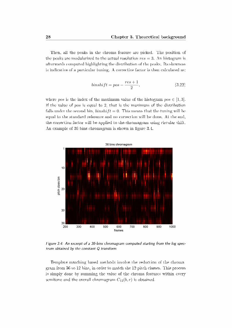
3.4 An excerpt of a 36-bins chromagram computed starting from
the log spectrum obtained by the constant Q transform . . . 28
3.5 An excerpt of a chromagram computed starting from the 36-
bins chromagram summing the values within each semitone. . 29
3.6 The sigmoid function is used for Logistic Regression. . . . . . 32
3.7 The gure shows a simple 2-dimensional example of appli-
cation of SGD. Starting from a random initialization of the
parameters their value is updated moving towards the direc-
tion specied by the gradient of the loss function. The random
initialization can result in a local minimum convergence. For
probabilistic models, however, it is not desirable to end in a
global minimum since in that case there would be overtting
of the training distribution. . . . . . . . . . . . . . . . . . . . 33
3.8 The graphical representation of a one hidden layer multilayer
perceptron withM input units, H hidden units and K output
units . . . . . . . . . . . . . . . . . . . . . . . . . . . . . . . . 36
3.9 The Restricted Boltzmann Machines are composed by a vis-
ible layer x and a hidden layer h where every input unit is
connected to every hidden unit by means of bidirectional ar-
rows. . . . . . . . . . . . . . . . . . . . . . . . . . . . . . . . . 40
IX

3.10 The Deep Belief Network is treated during the pretraining
phase as a generative model with a Restricted Boltzmann Ma-
chine on top. Each pair of layer is trained separately consid-
ering it as a RBM, each time propagating upwards the ac-
tivations of the hidden units. This allows to obtain better
initialization of the parameters. . . . . . . . . . . . . . . . . . 43
3.11 During the netuning and classication phases, the Deep Be-
lief Network is treated like a Multi Layer Neural Network, a
discriminative model. The netuning is done using Stockas-
tic Gradient Descent with backpropagation of the errors, the
classication is simply done by means of a forward pass of the
network. . . . . . . . . . . . . . . . . . . . . . . . . . . . . . . 44
4.1 The chord transcription process involves two main phases. A
feature extraction phase where the chromagram is extracted
from the audio signal and processed. The subscript β indi-
cates the number of bins of the chromagram that, in our case,
will be of 12 or 36 depending on the classication method
used. The second phase is the classication phase, where the
chromagram is used as a feature to compute the classication
obtaining a chord label vector. . . . . . . . . . . . . . . . . . 47
4.2 The feature extraction phase aims to extract a good feature
from the audio signal. The standard baseline involves three
main steps that in the gure are shown as black blocks. The
possible variation of the standard process are shown as gray
blocks. These possibilities include the extraction of harmonic
components using HPSS, the A-weighting of the log spectrum
and ltering stages. At the end of the process the 12-bin
chromagram used by template-matching methods is obtained.
In our approach we used the 36 bins chromagram C36(b, r) as
input feature to the machine learning classiers. . . . . . . . . 49
4.3 The result of the application of the low-pass lter to a chro-
magram excerpt. . . . . . . . . . . . . . . . . . . . . . . . . . 52
4.4 The result of the application of the median lter to a chroma-
gram excerpt. . . . . . . . . . . . . . . . . . . . . . . . . . . . 53
4.5 The result of the application of the geometric mean lter to a
chromagram excerpt. . . . . . . . . . . . . . . . . . . . . . . . 54
4.6 The result of the application of the harmonic mean lter to a
chromagram excerpt. . . . . . . . . . . . . . . . . . . . . . . . 55
X
4.7 The chord classication using machine learning techniques is
based on the training of the classiers starting from a dataset
of labelled songs. The best model obtained is used to clas-
sify new unseen audio les whose chromagrams have been ex-
tracted and normalized. The no chord recognition as well as
a ltering stage is done separately after the classication. . . 58
4.8 The gure shows the learning process of the machine learning
classiers. At every epoch the Stochastic Gradient Descent
updates are computed starting from the parameters of the
model obtained at the previous epoch. At the beginning the
parameters are randomly initialized. Each time the model is
evaluated computing the classication errors on the evaluation
set. The parameters of the model that gave the minimum error
is used for the classication. . . . . . . . . . . . . . . . . . . 65
4.9 The gure shows the binary template model for the C major
chord, where the pitch classes corresponding to the notes be-
longing to the chord have value 1, the remaining have value
0 . . . . . . . . . . . . . . . . . . . . . . . . . . . . . . . . . . 72
5.1 This gure shows an example of computation of the RCO. In
this case the transcription found a wrong chord that is not
present in the ground truth annotation. The detected correct
chords remain overlapped for 7 time instants over 10 that is
the total duration. . . . . . . . . . . . . . . . . . . . . . . . . 74
5.2 In this plot each point represent a song where the mean har-
monicity and the best number of iterations of the HPSS algo-
rithm are shown. A correlation between these two variables
is not evident. The most of the songs have best performances
when 25 iterations are done. . . . . . . . . . . . . . . . . . . . 77
XI
5.3 The gure shows a comparison between the 12 bin chroma-
gram, that is the feature used by the template-matching ap-
proaches, and the feature extracted by the DBN after the pre-
training stage on the same excerpt of a 36 bins chromagram.
The vertical lines indicate a chord change. The dimension of
the feature is dependent on the dimension of the network, in
this case all the layers have 50 hidden units. In this case some
units are not activated, that corresponds to have a dark color,
while other are frequently activated, that corresponds to have
a bright color. Even if the interpretation of the extracted fea-
ture is not straight-forward, vertical blue lines highlight that
the characteristics of the feature change in correspondence to
chord changes. . . . . . . . . . . . . . . . . . . . . . . . . . . 83
5.4 The variation of the WAOR scores about every song in the
mixed 3 dataset. The result show that every method per-
formed dierently on each song without a techniques that
always performs better. The DBN, however, obtained the
highest weighted average score. . . . . . . . . . . . . . . . . . 85
5.5 The variation of the segmQ scores about every song in the
mixed 3 dataset. Like the WAOR case, the methods per-
formed dierently on each song. Also in this case the DBN
obtained the highest weighted average score. . . . . . . . . . . 86
5.6 The confusion matrix for DBN with Gaussian input units on
the Mixed dataset MIXED 4. The gure shows how the dif-
ferent chords has been classied by the DBN. A light color
means a high number of elements, vice versa a dark colors
corresponds to low number of elements. If a square is white
it means that all the chords have been successfully classied. . 87
5.7 The confusion matrix for the MLP on the best performing
dataset on the Mixed dataset MIXED 4. . . . . . . . . . . . . 88
5.8 The confusion matrix for the Logistic Regression on the best
performing dataset on the Mixed dataset MIXED 4. . . . . . 88
5.9 The gure shows how the WAOR score is inuenced by the
change of the training set cardinality. Even when the number
of elements is strongly reduced the score is close to 0.6. The
machine learning approach thus is robust to the training set
cardinality . . . . . . . . . . . . . . . . . . . . . . . . . . . . . 89
XII

5.10 The gure shows a comparison between the distribution of the
elements in the three datasets used for the Extended Training
Dataset experiment. The distribution of the elements is biased
towards the most frequent chords of each author. . . . . . . . 90
5.11 The gure shows the distribution of the elements in The Beat-
les training sets before and after the extension. The number of
major chords elements remain higher after the extension due
to the presence of more major chords in the original dataset. 91
5.12 The gure shows the distribution of the elements in the Robbie
Williams training sets before and after the extension. . . . . . 92
5.13 The gure shows the distribution of the elements in the MIXED
4 training sets before and after the extension. . . . . . . . . . 92
XIII

XIV

List of Tables
3.1 Correspondence between frequency ratios and musical interval
in equal temperament. . . . . . . . . . . . . . . . . . . . . . . 17
3.2 Pitch classes and their names. ] and [ symbols respectively
rise and lower the pitch class by a semitone. . . . . . . . . . . 17
3.3 This table shows the relation between pitches and their fre-
quency in the equal temperament using the standard reference
frequency A4 = 440Hz. . . . . . . . . . . . . . . . . . . . . . 19
5.1 The table shows the performances obtained by the chroma-
grams without any applied lter. . . . . . . . . . . . . . . . . 77
5.2 The table shows the performances obtained by the chroma-
grams with a ltering phase computed on the 36 bins repre-
sentation before the folding to 12 pitch classes. The averaging
lter is denoted as Avg, the median lter as Med, the geomet-
ric mean lter as Geom and the harmonic mean as Harm Mean. 78
5.3 The table shows the performances obtained by the chroma-
grams with a ltering phase computed on resulting 12 pitch
classes representation. . . . . . . . . . . . . . . . . . . . . . . 79
5.4 Comparison between the test error performances obtained by
a DBN with Gaussian input units on a randomly created spec-
trum frames, 36 bins chroma vectors and 12 bins chroma vec-
tors datasets. . . . . . . . . . . . . . . . . . . . . . . . . . . . 80
XV

5.5 The table shows the comparison between the performances
obtained with the dierent normalization strategies by the
machine learning approaches. Where no star is present, the
DBN did not have a pre-training stage. The (*) indicates
that the DBN has been pre-trained having Gaussian input
units, the (**) indicates that has been pre-trained having bi-
nary units. The L-∞ norm is described in Section 4.2.1, FS1
and FS2 are the rst and second methods described in Sec-
tion 4.2.1, STD is the standardization (section 4.2.1), BIN the
binarization (section 4.2.1). . . . . . . . . . . . . . . . . . . . 81
5.6 The table shows a comparison between the performances ob-
tained by the dierent methods considering dierent mixed
random datasets (MIXED 1, MIXED 2, MIXED 3, MIXED
4, MIXED 5), highlighting the best performing method for
each dataset. . . . . . . . . . . . . . . . . . . . . . . . . . . . 84
5.7 The table shows the performances obtained by the dierent
methods considering songs taken from the Beatles dataset
(TB) and Robbie Williams dataset (RW) highlighting the best
performing method for each dataset. . . . . . . . . . . . . . . 87
5.8 The table show the results obtained after the extension of the
training set using ETD strategy. With the extended datasets
there has been an improvement on the performances. . . . . . 91
XVI

1

2

Chapter 1
Introduction
With the diusion of the Internet and the growing availability of multimedia
content, in the past few years there has been an increasing need of developing
intuitive and innovative techniques to handle the big amount of information
available. Music has been strongly involved in this technological innovation,
particularly thanks to the evolution of the digital audio format. In fact,
due to the easiness of downloading, uploading and, in general, sharing the
music brought by the Web, the amount of musical content available has
dramatically increased over the last years. In this context, the need of music
information retrieval and classication systems has become more urgent and
this brought to the birth of a research area called Music Information Retrieval
(MIR). MIR is an interdisciplinary science with the main goal of retrieving
information from music. The interdisciplinarity comes from the need of a
background in both signal processing and machine learning techniques, but
also in musicology, music theory and psychoacoustics and even in cognitive
psychology and neurology. The Automatic Chord Recognition (ACR) task
is one of the main challenges in MIR.
The main goal of ACR is to obtain the transcription of the chord succession
that represents the harmony of a song in an automatic fashion. The notion
of chord is a well known concept in the music theory and it is, in general,
referred to the simultaneus execution of three of more notes. The concepts
regarding the musical background will be explained in detail in section 3. An
ACR system is able to analyze a piece of music and to give out a sequence of
labels that are associated to the chord progression played in the song. The
information brought by an ACR system is very useful both for didactic and
research purposes.
From the didactical point of view, it can be used by students of musical
instruments to retrieve chords of a song and in order to verify if his own
3
4 Chapter 1. Introduction
transcription is correct. In general, it can also be useful to automatically
produce musical sheets. Nowadays, many sites on the Internet oer the
possibility to download manually generated transcriptions posted by some
users, that can be musicians or even not. These transcriptions are, in many
cases, not very accurate. This can represent a problem for the not trained
musician and a waste of time for the trained one that has to invest some time
in retrieve his own transcription. The majority of the songs, however, do not
even have a transcription available online, thus an automatic transcription
system can be very useful for these needs.
From the research point of view, the chord succession can represent a
descriptor of an audio le that can be used in other MIR systems. The easiest
way to perform this task is to use metadata, like tagging, that have been
previously associated with songs. The accuracy of this approach, however,
is strongly related to the precision and the prociency of tagging that is
hand-made done by humans. Recently, therefore, the main goal of MIR
researchers has been to develop algorithms able to overcome this limitation
performing content-based information retrieval. With this approach, the
nal system must be able to extract meaningful information from an audio
signal trying to limit the intervention of the human being. This is done
applying both signal processing and machine learning techniques in order
to create algorithms that are able to automatically analyze the audio signal
and to perform the needed classication without using any human-made tag.
The ACR is an example of content based music information retrieval task.
The content based MIR systems, in general, follow a precise computa-
tional paradigm. It involves two distinct phases: in the rst one the goal
is to extract meaningful descriptor from the audio signal. This phase is re-
ferred as feature extraction. The main kind of features initially used were
the Low Level Features (LLF). They are directly extracted from the audio
signal using signal processing techniques and mathematical calculus. How-
ever, since music has a strong hierarchical structure, the features extracted
with this methods lack of semantic expressiveness. Researchers in MIR eld
have concentrated their eort on designing new kind of feature that can be
closer to the human way of thinking. The Mid Level Features (MLF) are
derived from LLF taking into account theoretical knowledge of the context.
They provide, just to give some examples, descriptors for melody, harmony
and rhythm. The High Level Features (HLF) are the closest to the human
way of thinking and they are semantically more informative for the human
being than the LLF and MLF. These are derived from LLF and MLF using
machine learning approaches or complex systems specically designed. The
whole automatic chord classication system, if inserted as part of another

5
MIR application, can be seen as a mid-level feature extractor. From this
point of view, chords can be used as features in other applications. For ex-
ample it can be used in a Music Emotion Recognition system. Music, in fact,
is the medium used by the composer to convey emotions to the listener and
thus the harmony of a song can be strongly related to mood. This intuition
is confermed by researches made in the psychoacoustical eld [38] where it
has been showed that some harmonic patterns can cause a physical response
in the human being. The relations between chords and other characteristics
of a musical piece like mood, however, is still a research area in MIR.
Emotions are not the only aspect linked to having specic chords pat-
terns. Also cover song retrieval and automatic genre classication could be
improved by having a good chord transcription available. It can be found,
in fact, recurrent harmonic patterns typical of a specic genre. In the blues
genre, for example, a standard pattern often used consists in the succession
respectively of the rst, fourth, rst and fth grades of the tonal key.
The ACR systems follow the paradigm usually used by MIR systems de-
scribed above. It requires a feature extraction phase and a classication
phase. The feature extraction is crucial in every MIR framework, since low
quality features can worsen the nal result, and it represents a bottleneck
to the entire process. In the second phase, probabilistic models or machine
learning techniques are used in order to handle the information brought by
the features previously extracted.
As we will deepen in the following chapter, in the existing systems there
are two main ways of computing a chord classication. A rst approach is to
compute a measure of distance between the extracted descriptior and a set
of templates. This method has the advantage that it does not depend from
a training phase and, therefore, from an accurate and comprehensive ground
truth dataset. On the other hand, template based approaches bring to poorer
results. Another approach is to add temporal probabilistic models of chords
and, in some cases, keys transitions. This approach can improve the quality
of the classication, but it has the drawback of being computationally more
expansive. In this thesis we explored the potential of the machine learning
classication methods when used to directly classify frames of the extracted
feature with respect to the straightforward template based methods. We
compared a linear model and a nonlinear model, logistic regression and single
layer perceptron, with the more recent Deep Belief Networks, reaching better
results in classication than the standard template matching approaches. We
also compared dierent techniques for the feature extraction phase with the
goal of improving the quality of the extracted descriptor
1.1 Thesis outline
In the next chapter we will review the main techniques in the state of the art
of Automatic Chord Recognition. The third chapter will give a theoretical
background of the most important concepts needed to understand this thesis.
In the fourth chapter we will describe our approach to the problem. The last
two chapter, 5 and 6, will focus respectively on the experimental results and
on conclusions and future works.
Chapter 2
State Of Art
In this chapter we will give an overview of the main existing techniques re-
garding Automatic Chord Recognition. Generally, the standard approaches
to the ACR problem always contain two main steps:
• a rst step where a robust low level feature is extracted and processed
in order to improve its quality;
• a second step where the chord classication is computed starting from
the extracted low level feature.
The techniques dier from each other with respect to the way in which these
steps are performed and to the methods used.
Regarding the rst step, the commonly extracted feature is a 12 dimen-
sional representation of the audio signal called chromagram (that will be
described in detail in chapter 3). The techniques dier from each other with
respect to the ways of doing denoising and pre or post-processing of the
chromagram. They will be reviewed in section 2.1.
Regarding the classication phase, the state of the art techniques can
be grouped into two families of approaches. The rst category groups all
the methods that exploit probabilistic models of the musical context, the
second category regards all the approaches that takes in consideration just
the direct classication of each song frame per se. Our work falls in this
second category. The main methods belonging to both the categories will be
reviewed in section 2.2.
In order to give a full review of the state of the art, this chapter is divided
in three main sections. In the rst one we will review the state of the art
approaches regarding the feature extraction phase. In the second section we
will focus on the classication phase reviewing all the main techniques. In
7
8 Chapter 2. State Of Art
the last section nally we will give an overview of the use of the deep learning
techniques in ACR.
2.1 Feature Extraction
The rst step performed in a chord recognition system is the extraction a
meaningful feature from the audio signal. This is a crucial phase since the
quality of the extracted feature inuences the performance of the entire sys-
tem. In the signal processing area there are various possible representation
of an audio signal that can be used for a classication problem like the ACR.
For example low level features like the Fourier Transform or the MFCCs can
be used. They, however, bring little semantic information needed for the
ACR task. For this reason, it is not convenient to use them directly as audio
descriptors to compute the chord classication. Instead, starting from the
computation of the Fourier Transform, the feature extraction process ends
with the creation of a more informative low level feature called chromagram
or Pitch Class Prole (PCP). The use of this kind of feature has been in-
troduced by Fujishima in [10] that developed the rst Chord Recognition
System.
The chromagram provides a musically-meaningful description of audio sig-
nal that, in our case, can be useful to nd the most probable chord that is
being played. The nal result of the process is a pitch class versus time rep-
resentation of the musical signal. The notion of pitch class is related to the
human way of perceive pitch and it will be deepen in Chapter 3. Fujishima
in [10] computed this feature starting from the DFT of the audio signal to be
analyzed. Another common method for chromagram computation involves
instead the use of the constant Q-transform [7] for the extraction of a log
frequency spaced spectrum, and it has been introduced for the chord recog-
nition task by Bello and Pickens in [3]. This process creates a log-spectrum
where the frequencies are not linearly spaced like in the STFT and for this
reason are closer to the frequency resolution of the human ear. The log spec-
trum is then folded to obtain a representation that highlights the 12 pitch
classes. The overall procedure will be explained in detail in Chapter 3.
Unfortunately, the chromagram suers of some problems. The main is-
sue regarding this kind of representation of the audio le is the presence of
noise in the computed spectrum. It is mainly due to the energy associated
to frequencies that do not actually correspond to the notes of the chord
that is being played. This energy can come from the presence of sources of
inharmonic sounds with a broadband spectrum, like drums, and from the
harmonics of an harmonic sound. The latter enrich the timbre of an in-
2.1. Feature Extraction 9
strument but are useless in ACR task, since they create false positive notes
in the chromagram itself. For the purpose of overcoming these limitations,
researchers tried to develop processing strategies aimed to make this feature
more robust to noise.
2.1.1 Feature processing
In the literature there are dierent ways of facing up to both of the prob-
lems previously described. Ni, McVicars [29] proposed to use the harmonic
components extracted by the Harmonic Percussive Signal Separation (HPSS)
algorithm introduced by [30] to compute the chromagram instead of using
directly the STFT of the audio signal. The HPSS algorithm performs a
separation of the harmonic and percussive components of an audio signal
based on the anisotropy of their spectra. This algorithm will be reviewed in
detail in Chapter 3. They also proposed a log10 based version of the chroma-
gram, called Loudness Based Chromagram, followed by A-Weighting. This
is motivated by the fact that the perceived loudness is approximately linearly
proportional to the sound pressure level. Khadkevic, Omologo computed a
chromagram starting from a reassigned spectrogram using Time Frequency
Reassignement [24]. This technique is used before the folding to 12 pitch
classes and brings to the creation of a Reassigned Chroma. As a result the
spectral representation becomes sharper, and this allows to derive spectral
features with higher time and frequency resolution. Glaziryn in [12] performs
a chroma reduction using DCT setting to zero the rst 10 resulting coe-
cients. He then applied a smoothing using self-similarity matrix. Another
way of reducing the amount of the undesirable harmonic components is to
create two pitch salience matrices, one considering a simple tone and the
other considering also harmonics in a geometric sequence. The noise reduc-
tion is obtained retaining only peaks in both salience matrices [15] [27].
Temporal continuity and feature denoising is enforced by the use of median
or low pass ltering on the time axis. In this way temporal correlation
between chroma vectors is also exploited [32]. An appropriate length of the
lter has to be chosen taking into account the trade o between the presence
of percussive transients and rapidly changing chords. Beat synchronization
of the chromagram is also often performed, replacing every chroma vector
with the median of the vectors between two beat intervals [3]. The main
drowback of this approach is that the accuracy of doing beat synchronization
is dependent on the performance of the beat tracker.
Another fact that has to be taken into account is that the tuning of the
instruments performing in a song can inuence the correctness of the chro-
10 Chapter 2. State Of Art
magram. The standard reference for tuning the central A4 frequency in the
western musical world is 440Hz. This value, however, can change and fall in
the range of 415Hz to 445Hz. For this reason it is necessary to determine
it and modify coherently the chromagram. The main approach creates a
spectrum with a higher resolution than needed, in general 3 bins per semi-
tone. Starting from this feature, a possible approach is to apply parabolic
interpolation or circular statistics to nd the position of the peak of the dis-
tribution. In this way the shift from the central bin is found, and it is then
possible to shift the reference frequency [16].
2.2 Classication
Once the feature has been extracted it is used to compute the chord clas-
sication phase. As we mentioned at the beginning of the chapter, the ap-
proaches regarding this phase can be divided in two main categories that
will be addressed in the following subsections.
2.2.1 Template-Matching Classication
The rst category groups the methods that do not make use of probabilistic
models in order to model chord transition probabilities. The simplest way
to nd out the candidate for a chord in a specic time slice is based on a
template-matching procedure. These methods are called template-matching
approaches. They are based on the creation of models of template chroma
vectors that represent all possible chords. The most common chord template
vector is a 12 dimensional binary vector with the elements corresponding
to the notes of the chord set to 1. The remaining elements are set to 0
[32]. Once the model has been created, a measure of distance or similarity
between each chroma vector and each created chord template is then applied
in order to nd the most similar chord. This measure of similarity is used
to compute the classication in the template-matching based approaches
[32], but it is also used as observation of a probabilistic model by the music
theory based approaches [2]. In order to improve the quality of the model,
Glazyrin [12] emphasized the elements corresponding to the rst and the fth
note of the chord, normalizing them to have unit length in the Euclidean
space. Chen et al [8] created a 24 dimensional template with the rst 12
dimensions representing the bass note and the successive 12 corresponding
to the standard chord label.
Regarding the choice of the similarity measure, the rst measure that has
been used in the literature is the simple inner product introduced by Fu-

2.2. Classication 11
jishima in the rst chord recognition system [10]. Successively other metrics
have been applied. In particular, the most used measures of distances are
the Kullback-Leibler divergence, together with the Itakura-Satio distance
and the Euclidean distance [31]. In their study Oudre et al in [31] proved
that the Kullback-Leibler divergence is the best performing one. Again
Oudre in [33] enhanced the template-matching based approach introducing
an Expectation-Maximization algorithm to identify a priori chord probabil-
ities. In this thesis we explored how machine learning techniques can be
used directly as classiers, overcoming the problem of creating a model of
templates of chroma vectors and the choice of a measure of distance.
Within a song, chords remain usually stable for a certain period of time.
The presence of noise in the spectrum, can inuence the correctness of certain
chroma vectors. It is necessary, thus, to nd a way to isolate the outliers in
order to smooth the obtained chord progression. The strategy used by these
kind of methods is to lter the chromagram in the time domain, in order to
smooth the resulting representation. The two main lters used are the low
pass and the median lter [32]. In this thesis we explored the use of other
two kind of lters, geometric mean and harmonic mean. The main advantage
of using a lter to exploit temporal correlation is that this approach does
not depend on a training phase or a creation of a state transition model by
a musical expert. This method is, thus, more exible even if less accurate.
2.2.2 Probabilistic models of chord transitions
The other family of approaches make use of probabilistic models containing
state transition distributions. This allows to penalize state transitions with
low probability obtaining a gain in the classication performance. The chord
transitions probabilities can be obtained from a training stage considering
a training set of songs, in this case this kind of approaches are data driven.
The other option is to x a priori probabilities considering music theory and
perception. In this second case the use of an expert musician is required.
The most used probabilistic model within this category of approaches is
the Hidden Markov Models (HMMs). The HMMs can model sequences of
events in a temporal grid considering hidden and visible variables. They,
however, can take into account just one hidden variable. In the case of
chord recognition, the hidden states correspond to the real chords that are
being played, while the observations are the chroma vectors. The chroma
distributions are mainly based on the chord proles. Hidden Markov Models
are used in [3], [34].
In order to add the capability of model other characteristics of the song, in

12 Chapter 2. State Of Art
[27] the use of Dynamic Bayesian Networks has been introduced. They are
an extension of the HMMs that allows to model also other parameters, like
the key or the bass note and, thus, they improve the expressiveness of the
model. The goal is to enlarge the point of view regarding the classication
approach including also information coming from the musical background.
In this way the model of the context is further enriched allowing to obtain a
more comprehensive model that has the eect to improve the classication
accuracy.
2.3 Deep Learning in Chord Recognition
Deep architectures are machine learning techniques that have had a great
development in the past few years. They are composed of many layers of non-
linear operations and they are particularly suited to learn the complicated
functions that represent high level abstractions. For this reason the use
of deep architectures in many areas of computer science and engineering is
growing exponentially. The theoretical concepts and the detailed description
of deep architectures will be explained in Chapter 3. Just recently, the
researchers in MIR eld started to investigate the use of deep architectures
for MIR tasks. The reasons behind this research trend can be seen as a
reaction to two main problems.
As we mentioned before, the main issue in content based information re-
trieval is the design of robust and informative features. Music content based
analysis is not an exception, and the performances of the techniques regard-
ing this research area are highly dependent on the quality of the feature
extraction phase. At the moment feature representations are, in most of
the cases, heuristically designed making large use of knowledge of context
domain information coming from music theory to psychoacoustics. The 12
dimensional representation of the musical signal used in chord recognition
is an example of this fact. As argued by Bello et al in [23] the limitations
of a hand-crafted feature extraction process can be summarized in dierent
problems. The rst reason comes from the fact that the data representation
used imposes an upper bound on the best possible semantic interpretation
that will be dependent on the feature quality. The need for complex semantic
interpretation methods can be strongly reduced by the improvement of the
feature representation. Finally, having hand made features brings the prob-
lem that they are not scalable to domains that have dierent characteristics
with respect to the one where they have been thought. Their application is,
thus, limited to the area that they have been designed to cover.
The other important motivation of this change is that music has a strong

hierarchical structure. Notes, in fact, are just in the lower level element of
the musical perception. They are combined to create larger units like chords
and phrases. Phrases are combined in musical movements like verses and
choruses, and all these elements together are part of the highest levels of ab-
stractions that includes the concepts of musical genre or even the subjective
eld of emotions. Deep architectures have been introduced also with the goal
of modeling the hierarchical way of organize information of our brain. For
these reasons, the use of deep architectures for automatic feature extraction
and classication in MIR, that deals about a very hierarchical element like
music, could have a good impact. Deep learning techniques, however, are
not exempt from problems. The main issues regarding these models is the
diculty of doing the training phase of the generative probabilistic models
used by deep techniques (these concepts will be deepen in Chapter 3).
Regarding automatic chord recognition, the use of deep learning is still at
the early research phases. The main applications of these techniques in the
literature regards the use of Convolutional Neural Networks (CNNs) and De-
noising Autoencoders (DAs) for automatic feature extraction. In [22] Bello et
al use CNNs to learn a function that projects audio data into Tonnetz-space.
In [13] Glazyrin uses Stacked Denoising Autoencoders to extract Mid Level
Features for chord estimation. Again Bello and Humphrey in [22] proposed
the rst application of deep techniques for classication. They use CNN to
classify ve seconds tile of pitch spectra, obtaining performance competitive
to the standard techniques.
In this thesis we used Deep Belief Networks with greedy layer-wise pre-
training and Neural Networks directly as classiers for the Chord Recognition
Task. We tested their performance when they are used to classify vectors of
the chromagram and we compared the results with a linear classier and the
state of the art template-matching based approaches obtaining competitive
results.

14 Chapter 2. State Of Art

Chapter 3
Theoretical background
This chapter will focus on the theoretical concepts needed to understand our
work. First of all we will review the basic musical concepts, in particular we
will describe the notions of chords and pitch classes. We will see also how
the main scales can be harmonized. In the second section we will explain
the signal processing techniques used to extract the mid level feature used in
the chord recognition process. In particular, we will focus on the Short Time
Fourier Transform (STFT) and the algorithm of Harmonic Percussive Signal
Separation (HPSS). We will see, then, the way in which the chromagram is
computed using the Constant Q-Transform. The last section is dedicated to
the machine learning algorithms that we used as the classication methods.
We will review the concepts behind the Logistic Regressor and the Multi
Layer Perceptron Neural Network (MLPNN). At the end, we will explain in
detail the concepts behind the Deep Belief Networks (DBNs)
3.1 Musical background
This section will focus on the main concepts from music theory that are
needed for the comprehension of the study. First, we will explain the no-
tion of pitch and pitch classes. We will then expound the concept of chord
and how dierent chords can be constructed. The concepts in the following
sections can be reviewed in more detail in [11], [36], [26]
3.1.1 Pitch and Pitch Classes
Pitch is the perceptual attribute that is used to describe the subjective per-
ception of the hight of a note. It is the attribute that allows humans to
organize sounds on a frequency-related scale that ranges from low to high
sounds [25]. Thanks to this perceptual cue, we are able to identify the notes
15
16 Chapter 3. Theoretical background
on a musical scale. Along with duration, loudness and timbre it is one of
the major auditory attributes of musical sounds. Since it is a psychoacoustic
variable, the pitch perception depends on subjective sensitivity.
In the simplest case of a sound with a single frequency (i.e. a sinusoidal
tonal sound), the frequency is its pitch [39]. In general, almost all natural
sounds that give a sensation of pitch are periodic with a spectrum (the
concept of spectrum will be described in 3.2.1) made by harmonics that are
integer multiples of a fundamental frequency. The perceived pitch in these
cases, correspond to the fundamental frequency itself. Humans, however, are
also able to identify a pitch in a sound with an harmonic spectrum where
the fundamental is missing, or even in presence of inharmonic spectra.
In the past few years, dierent theories have been proposed to explain
the human pitch perception process [39], but it's still not completely clear
how the pitch is coded by human brain and which factors are involved in the
perception.
In music, phenomenon of pitch perception brought to the denition of the
concept of notes that are associated to perceived frequencies. The distance
between two notes is called interval. Nowadays, the common musical tem-
perament used for the instruments tuning is the equal temperament, where
every pair of adjacent notes has an identical frequency ratio. In this way
the perceived distance from every note to its neighbor is the same for every
possible notes. The perceived pitch is proportional to the log-frequency. In
this system, every doubling of frequency (an octave) is divided into 12 parts:
fp = 2112 fp−1 (3.1)
where fp is the frequency of a note, fp−1 the frequency of the previous note.
According to this temperament, the smallest possible interval between two
notes corresponds to the ratio
fpfp−1
= 2112 (3.2)
that it's called semitone. The relations between frequency ratios and musical
intervals are showed in Table 3.1.

3.1. Musical background 17
Frequency Ratio Musical Interval #
1 Unison
2 Octave
2912 = 1.682 Major Sixth
2812 = 1.587 Minor Sixth
2712 = 1.498 Fifth
2512 = 1.335 Fourth
2412 = 1.259 Major Third
2312 = 1.189 Minor Third
2112 = 1.059 Semitone
Table 3.1: Correspondence between frequency ratios and musical interval in equal tem-
perament.
note name pitch class #
C 1
C]/D[ 2
D 3
D]/E[ 4
E 5
F 6
F]/G[ 7
G 8
G]/A[ 9
A 10
A]/B[ 11
B 12
Table 3.2: Pitch classes and their names. ] and [ symbols respectively rise and lower
the pitch class by a semitone.
An important perceptual aspect that must be taken in consideration is
that human pitch-perception is periodic. If two notes are played following a
unison interval, that corresponds to have the same fundamental frequency,
the perceived pitch is the same. While if two notes are in octave relation, that
corresponds to a doubling of frequency, the perceived pitches have similar
quality or chroma. This phenomenon is called octave equivalence and brought
to the denition of the concept of pitch class. Human are able to perceive
as equivalent pitches that are in octave relation. This phenomenon is called
18 Chapter 3. Theoretical background
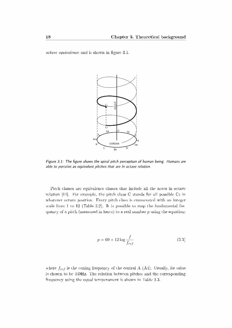
octave equivalence and is shown in gure 3.1.
Figure 3.1: The gure shows the spiral pitch perception of human being. Humans are
able to perceive as equivalent pitches that are in octave relation.
Pitch classes are equivalence classes that include all the notes in octave
relation [11]. For example, the pitch class C stands for all possible Cs in
whatever octave position. Every pitch class is enumerated with an integer
scale from 1 to 12 (Table 3.2). It is possible to map the fundamental fre-
quency of a pitch (measured in hertz) to a real number p using the equation:
p = 69 + 12 logf
fref(3.3)
where fref is the tuning frequency of the central A (A4). Usually, its value
is chosen to be 440Hz. The relation between pitches and the corresponding
frequency using the equal temperament is shown in Table 3.3.
3.1. Musical background 19
Octave
Note 2 3 4 5 6
C 66 Hz 131 Hz 262 Hz 523 Hz 1046 Hz
C]/D[ 70 Hz 139 Hz 277 Hz 554 Hz 1109 Hz
D 74 Hz 147 Hz 294 Hz 587 Hz 1175 Hz
D]/E[ 78 Hz 156 Hz 311 Hz 622 Hz 1245 Hz
E 83 Hz 165 Hz 330 Hz 659 Hz 1319 Hz
F 88 Hz 175 Hz 349 Hz 698 Hz 1397 Hz
F]/G[ 93 Hz 185 Hz 370 Hz 740 Hz 1480 Hz
G 98 Hz 196 Hz 392 Hz 784 Hz 1568 Hz
G]/A[ 104 Hz 208 Hz 415 Hz 831 Hz 1661 Hz
A 110 Hz 220 Hz 440 Hz 880 Hz 1760 Hz
A]/B[ 117 Hz 233 Hz 466 Hz 932 Hz 1865 Hz
B 124 Hz 247 Hz 494 Hz 988 Hz 1976 Hz
Table 3.3: This table shows the relation between pitches and their frequency in the
equal temperament using the standard reference frequency A4 = 440Hz.
3.1.2 Chords
With chord it is generally meant the simultaneous execution of three or
more notes. Two notes played together form a particular type of interval
called harmonic interval. Chords are made combining two or more harmonic
intervals in specic relations. They are classied considering the number of
notes that are being played and the type of the intervals. The most common
type of chord, that is the one that is more used in western pop music, is
called triad. It's made by 3 notes played together, that correspond to 2
thirds. The three notes that form a triad are:
• the root note;
• the characteristic or modal note;
• the dominant note.
Triads are formed by stacking one third on top of another. There are four
possible combinations:
• a major third with a minor third above makes a major triad ;
• a minor third with a major third above makes a minor triad ;
• two overlapping minor thirds make a diminished triad ;

20 Chapter 3. Theoretical background
• two overlapping major thirds make a augmented triad.
In the most general case, triads are shown in the root position, that is,
with the root note on the bottom. In practice, triads are often inverted.
This means that the chord has a note other than the root in the starting
position. However we will not dwell on these concepts since it is beyond the
scope of this thesis.
3.2 Signal processing tools
In this chapter we will focus on the theoretical background regarding the
feature extraction phase of the chord recognition process. The computation
of the mid-level feature used for the classication is based on the processing
of the audio signal by means of low level signal processing tools. First, we
will review the concept of Short-Time Fourier Transform (STFT) that is the
frame-wise computation of the Discrete Fourier Transform (DFT). The result
of this process is a frequency versus time representation of the signal that is
the starting point for the computation of the chromagram. We will, then,
see the method used to separate the harmonic and percussive components of
the audio signal. Finally, we will describe the simplest computation of the
chromagram starting from the output of the STFT.
3.2.1 Short-Time Fourier Transform
The Short-Time Fourier Transform (STFT) is computed applying the Dis-
crete Fourier Transform (DFT) to small segments of the audio le obtained
by a windowing process. The absolute value of the representation of the
audio signal obtained with the application of the STFT is also called spec-
trogram. The DFT is the relative of the Fourier Transform (FT) applied
to discrete-time signals. The Fourier Transform of a continuous-time signal
x(t) is dened as:
X(ω) =
∫ +∞
−∞x(t)e−jωtdt, ω ∈ (−∞,+∞). (3.4)
The DFT has similar denition to the FT, with the dierence that the quan-
tities have discrete values and, thus, the integral is replaced with a nite sum:
X(ωk) =N−1∑n=0
x(tn)e−jωktn k = 0, 1, 2, ..., N − 1. (3.5)
The DFT is simpler mathematically but more relevant computationally than
the FT since, in practice, signal and spectra are processed in sampled form
3.2. Signal processing tools 21
and x(tn) is always nite. The meaning of the quantities in the denition is
the following:
• x(tn) is the input signal at time tn;
• tn = nT , where T is the sampling interval in sec and n an integer ≥ 0;
• X(ωk) is the complex valued spectrum of x at frequency ωk;
• ωk = kΩ is the kth frequency sample in rad/sec;
• Ω = 2πNT is the radian-frequency sampling interval in rad/sec;
• fs = 1T is the sampling rate in Hz;
• N is the integer number of time samples.
In the literature, it is common to set T = 1 in the previous equation in order
to obtain tn = n. Both the signal x(n) and the transform X(ωk) are discrete
quantities represented by N samples. If, in the previous equation, we call
sk(n) = ejωnn (3.6)
the denition can be written like:
X(ωk) = 〈x, sk〉. (3.7)
The transform, thus, can be seen as a measure of similarity between a signal
x(n) and the complex exponentials sk(n). These are called basis functions.
The musical signal is highly non-stationary. The drawback of the DFT is
that the temporal information is lost. For this reason it is necessary to
compute a local analysis of the frequency components and not taking the
signal as a whole. This can be easily done computing the DFT on portions
of the signal, called frames, obtained multiplying the signal by a time sliding,
nite and zero phase window w(n). The parameters that must be specied
are:
• the size of the transform NFT ;
• the window length L that must be L ≤ NFT ;
• the hop-size Hop, that indicates the distance in samples between two
consecutive windows.

22 Chapter 3. Theoretical background
w(n) must be 6= 0 for 0 ≤ n ≤ Lw − 1. The formulation of the STFT is
written as:
Xstft(ωk, r) =
NFT−1∑n=0
(x(n− rHop)w(n))e−jωkn k = 0, 1, ..., NFT , (3.8)
The main drawback of using this method is that there is a trade-o between
temporal and frequency resolution. This is due to the fact that the multi-
plication in the time domain of the signal x(n) with the window w(n) corre-
sponds to the convolution between their spectra Xstft(ωk, r) and W (ωk, r)
in the frequency domain. The presence of the windows, thus, alters the
spectrum of the signal. The consequence is that two harmonics very close
in frequency can be distinguished only increasing the temporal amplitude
of the window. In this way there is a reduction of the temporal resolution,
that is the reason why the STFT has been introduced. In particular, the
frequency resolution ∆f is expressed as:
∆f =fsNFT
(3.9)
where fs is the sampling frequency of x(n). The window length must be
chosen taking into account what is the frequency resolution needed for the
specic problem. At the same time, if the window length is chosen to be
Lw = NFT = 2η the computational time of the DFT can be strongly re-
duced. In fact, by means of the Fast Fourier Transform algorithm, using this
value the computational complexity of the Transform becomes O(N logN).
Evaluating directly the denition of the DFT would have required O(N2)
operations, since there are N outputs and each output requires a sum of N
terms.
3.2.2 Harmonic Percussive Signal Separation
One of the main problems regarding the chords classication is the pres-
ence of noise in the audio signal coming from the presence of sounds with
inharmonic spectrum generated, for example, by percussive instruments. In
this section we will outline a method proposed by Ono, Miyamoto et all
in [30] which goal is to separate the harmonic and percussive components
of the spectrograms. As we mentioned in the previous chapter, the feature
used for chord classication is a pitch class versus time representation of the
audio signal called chromagram. The audio signal obtained from the har-
monic spectrum can be used as starting point for the computation of the
chromagram instead of using the original audio signal as proposed by [29].
3.2. Signal processing tools 23
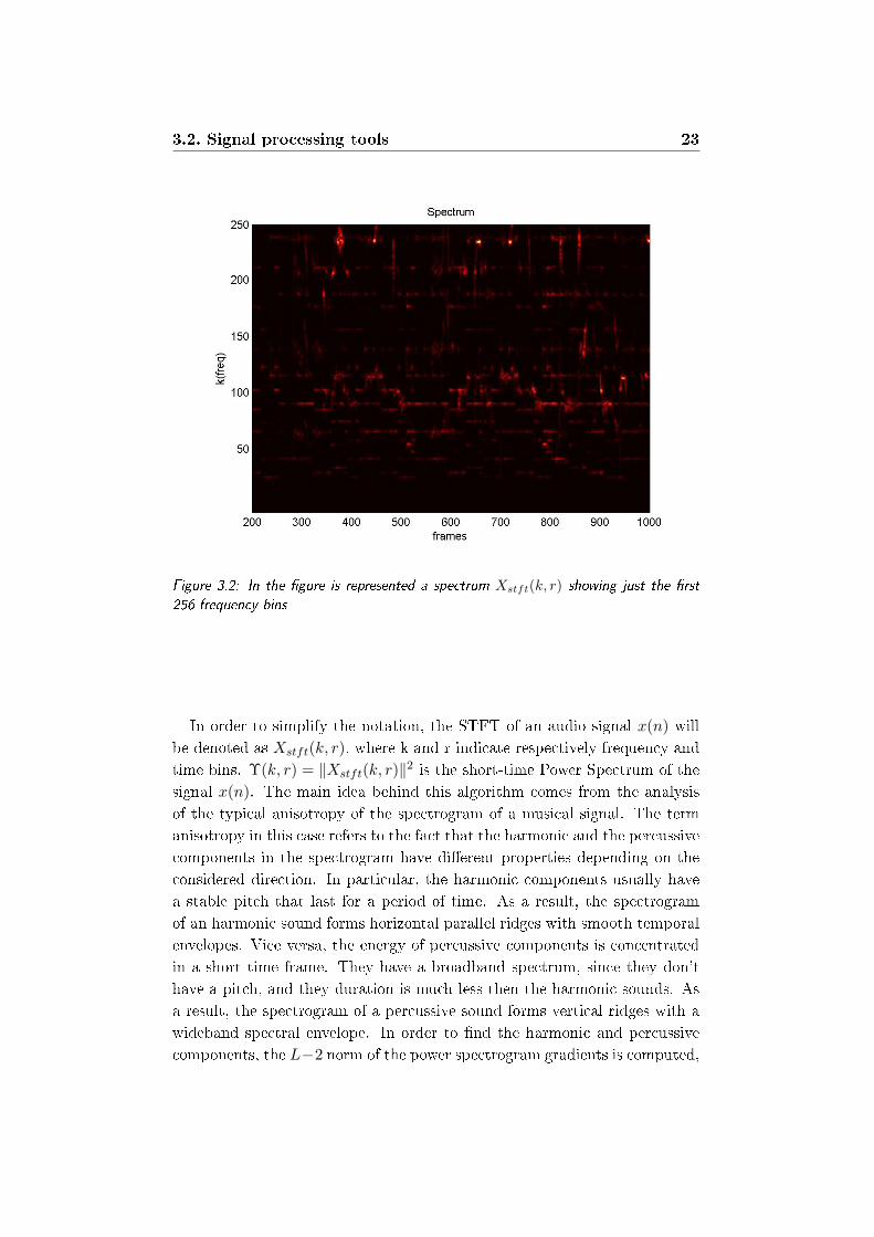
Figure 3.2: In the gure is represented a spectrum Xstft(k, r) showing just the rst
256 frequency bins
In order to simplify the notation, the STFT of an audio signal x(n) will
be denoted as Xstft(k, r), where k and r indicate respectively frequency and
time bins. Υ(k, r) = ‖Xstft(k, r)‖2 is the short-time Power Spectrum of the
signal x(n). The main idea behind this algorithm comes from the analysis
of the typical anisotropy of the spectrogram of a musical signal. The term
anisotropy in this case refers to the fact that the harmonic and the percussive
components in the spectrogram have dierent properties depending on the
considered direction. In particular, the harmonic components usually have
a stable pitch that last for a period of time. As a result, the spectrogram
of an harmonic sound forms horizontal parallel ridges with smooth temporal
envelopes. Vice versa, the energy of percussive components is concentrated
in a short time frame. They have a broadband spectrum, since they don't
have a pitch, and they duration is much less then the harmonic sounds. As
a result, the spectrogram of a percussive sound forms vertical ridges with a
wideband spectral envelope. In order to nd the harmonic and percussive
components, the L−2 norm of the power spectrogram gradients is computed,
24 Chapter 3. Theoretical background
and H(k, r) and P (k, r) are found by minimizing the cost function:
J(H,P) =1
2σ2H
∑k,r
(H(k, r−1)−H(k, r))2+1
2σ2P
∑k,r
(P (k−1, r)−P (k, r))2
(3.10)
under the constraints:
H(k, r) + P (k, r) = Υ(k, r) (3.11)
and
H(k, r) ≥ 0, P (k, r) ≥ 0. (3.12)
The meaning of the parameters is the following:
• H and P are sets of H(k, r) and P (k, r);
• σH and σP are horizontal and vertical smoothness control parameters.
With this formulation and under the assumption that the spectrograms gra-
dients follow independent Gaussian distribution, the problem leads to a sim-
ple formulation and solution. This assumption is not perfectly veried in
practice but an approximation can be found replacing the spectrogram with
a range-compressed version: Υc(k, r) = ‖Xstft(k, r)‖2γ with (0 ≤ γ ≤ 0).
The goal of the algorithm is to nd H(k, r) and P (k, r) as the elements that
minimize the cost function deriving a simple iterative solution. In order to
do this the algorithm adopts an auxiliary function approach that allows to
avoid the direct computation of the partial derivatives ∂J/∂H(k, r) = 0,
∂J/∂P (k, r) = 0. The detailed denition of the auxiliary function as well as
the detailed derivation of the update rules can be found in [30]. The nal
equations of the iterative algorithm at step i are:
H(k, r)i+1 = H(k, r)i + δi, (3.13)
P (k, r)i+1 = P (k, r)i + δi. (3.14)
The update parameter is equal to:
δi = α(H(k, r − 1)i − 2H(k, r)i +H(k, r + 1)i
4)−(1−α)(
P (k − 1, r)i − 2P (k, r)i + P (k + 1, r)i
4).
(3.15)
The overall updates are repeated for a xed number of iterationsNhpss. From
the harmonic spectrum H(k, r) the harmonic signal can be re-synthesised
obtaining xh(n) that can be used as starting point for the computation of
the low level feature used in ACR.
3.2. Signal processing tools 25
3.2.3 Q-Transform and Chromagram
Chromagram is a low-level feature that has been specically introduced for
musical-matching problems. The reason why this kind of feature has been
introduced rely on the poor semantic brought by other low level features
such as the Short Time Fourier Transform. The goal of the chromagram is
to highlight the contribution of every pitch class in terms of energy at each
time frame. As a result, a pitch-class versus time representation of the audio
signal is obtained. In this way, this information can be directly used in order
to nd the most probable chord that is playing at a certain time.
In the literature there exists dierent methods that have been used to
compute the chromagram. In this section we will show the basic computa-
tional steps that has been used by Bello and Pickens in [3] that is the feature
that we used in our work.
The steps for the computation of the chromagram are:
• compute the STFT of the audio le;
• obtain the chroma feature from the log-spectrum using the Constant
Q-Transform kernel;
• tune the chromagram with respect to the standard tuning reference
and reduce the number of bins to the 12 pitch classes.
STFT computation
The rst step in the computation of the chromagram is the extraction of the
STFT. This low-level feature is used in order to have a faster implementa-
tion of the constant Q-transform. As we saw in the previous section, the
parameters that need to be chosen are the window length and type and the
hopsize Hop. The rst consideration is that the signal can be down-sampled
without any loss of information. In fact, the frequencies of the notes be-
tween C0 and C7 have values in the range between 30 and 2000Hz. For this
reason, the signal can be down-sampled to 11025Hz. Regarding the choice
of the window length, it must be taken into account that:
NFT > ϑfs
|f2 − f1|, (3.16)
where f2 and f1 are the two closest frequency that have to be distinguished,
fs is the sampling frequency and ϑ is a parameter whose value depends on
the choice of the window type. In the case of Hamming window the value of
26 Chapter 3. Theoretical background
ϑ = 4 because of the wideness of its main lobe. In order to the A3 and G]3
can be distinguished, the constraints of the previous equation become:
NFT > 411025
|220− 208|= 3675. (3.17)
Constant-Q Spectral Transform
The main issue in the application of the Fourier Analysis in musical applica-
tions, lie in the fact that the frequency domain bins are linearly spaced. This
is due to the fact that the Transform is computed using a constant resolu-
tion and frequency dierence. The frequencies using the equal temperament
are, however, geometrically spaced. The DFT spectrum, thus, does not map
eciently to musical frequencies.
The Constant Q Spectral Transform (CQT) has been introduced by Brown
in [7]. The usefulness of the CQT relies in the fact that, with an appropriate
choice of the parameters, the center frequencies of the transformation directly
correspond to the ones of the musical notes. In addiction, the time resolution
of the CQT is increasing towards the high frequencies. This is similar to the
behavior of the human auditory system. The CQT has a denition similar
to the one of the DFT, with the dierence that the center frequencies are
geometrically spaced:
fk = f0 · 2kβ k = 0, 1, ... (3.18)
where k is the frequency index, f0 corresponds to the minimum frequency
and β is the number of bins per octave. The denition becomes:
Xcq(k, r) =1
Nk
∑n≤Nk
x(n− rHop)w(n)ej2πnQ/Nk , (3.19)
where Q = (21β − 1)−1 and Nk = dQ fs
fke.
The calculation of the CQT according to the previous formula is com-
putationally very expansive. Brown and Puckette [7] proposed an ecient
algorithm based on matrix multiplication in frequency domain. The formula
in matrix notation is:
Xcq =1
NXstft · S∗ (3.20)
where Xstft is the Short Time Fourier Transform of the signal x(n) and S
is the FFT of the temporal kernel of the CQT. Since the kernel is a sparse
matrix, it involves less multiplications than directly compute the denition
and speeds up the entire process.

3.2. Signal processing tools 27
Figure 3.3: A log spectrum obtained after the application of the constant Q transform
Chromagram computation
From the log-spectrum obtained by the application of the CQT, the chro-
magram can be computed for every frame as:
Cβ(b, r) =M∑m=0
|Xcq(b+mβ, r)|, (3.21)
with b ∈ [1, β] corresponds to the chroma bin, r to the time bin and M is
the total number of octaves considered in the CQT. The number of bins has
been chosen to be β = 36, corresponding to have 3 bins per semitone. This
higher resolution is necessary in order to do tuning in the next stage.
Tuning and folding to 12 pitch classes
It can happen in music that recordings are not perfectly tuned with respect
to the standard reference A4 = 440Hz. For this reason the position of
the energy peaks can be dierent from the one that is expected. Having a
resolution of 36 bins per octave allows to compute an interpolation that can
correct the error brought by the dierent tuning compensating the bias on
peak locations. A simple tuning process it has been proposed by Harte in
[17].
28 Chapter 3. Theoretical background
Then, all the peaks in the chroma feature are picked. The position of
the peaks are modularized to the actual resolution res = 3. An histogram is
afterwards computed highlighting the distribution of the peaks. Its skewness
is indicative of a particular tuning. A corrective factor is then calculated as:
binshift = pos− res+ 1
2, (3.22)
where pos is the index of the maximum value of the histogram pos ∈ [1, 3].
If the value of pos is equal to 2, that is the maximum of the distribution
falls under the second bin, binshift = 0. This means that the tuning will be
equal to the standard reference and no correction will be done. At the end,
the correction factor will be applied to the chromagram using circular shift.
An example of 36 bins chromagram is shown in gure 3.4.
Figure 3.4: An excerpt of a 36-bins chromagram computed starting from the log spec-
trum obtained by the constant Q transform
Template-matching based methods involve the reduction of the chroma-
gram from 36 to 12 bins, in order to match the 12 pitch classes. This process
is simply done by summing the value of the chroma features within every
semitone and the overall chromagram C12(b, r) is obtained.
3.3. Classication methods 29
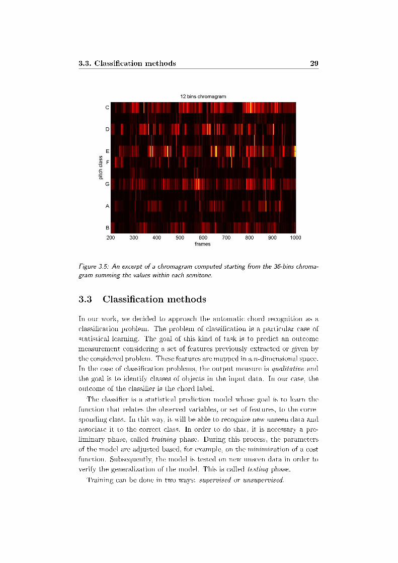
Figure 3.5: An excerpt of a chromagram computed starting from the 36-bins chroma-
gram summing the values within each semitone.
3.3 Classication methods
In our work, we decided to approach the automatic chord recognition as a
classication problem. The problem of classication is a particular case of
statistical learning. The goal of this kind of task is to predict an outcome
measurement considering a set of features previously extracted or given by
the considered problem. These features are mapped in a n-dimensional space.
In the case of classication problems, the output measure is qualitative and
the goal is to identify classes of objects in the input data. In our case, the
outcome of the classier is the chord label.
The classier is a statistical prediction model whose goal is to learn the
function that relates the observed variables, or set of features, to the corre-
sponding class. In this way, it will be able to recognize new unseen data and
associate it to the correct class. In order to do that, it is necessary a pre-
liminary phase, called training phase. During this process, the parameters
of the model are adjusted based, for example, on the minimization of a cost
function. Subsequently, the model is tested on new unseen data in order to
verify the generalization of the model. This is called testing phase.
Training can be done in two ways: supervised or unsupervised.
30 Chapter 3. Theoretical background
• in supervised learning the training phase is done knowing the correct
class (Ground Truth) of each input data;
• in unsupervised learning the parameters are adjusted observing only
the input distribution and no measurements of the outcome are pro-
vided.
The prediction in a classication problem takes values in a discrete set.
It is possible, thus, to divide the input feature space into a collection of
regions labeled according to the correct classication. The boundaries of
these regions can be rough of smooth depending on the prediction function
that links the input data to the corresponding classes. Statistical learners
can model linear or non-linear functions depending on the linearity or non-
linearity of these decision boundaries. In this section we present a linear and
two non-linear models that we tested in our specic classication problem.
From the statistical point of view, there is another distinction that can be
done concerning the goal of a learner. Given a generic input variable X and
an output variable Y.
• the generative models are designed to learn the joint distribution P (X,Y).
The conditional probability P (Y|X) can be obtained applying Bayes
rule; [18]. They are usually trained in an unsupervised manner;
• the discriminative models have the goal of modeling directly P (Y|X)
without caring about how the data was generated. They are usually
trained in a supervised manner.
3.3.1 Logistic Regression
Logistic regression is one of the most used discriminative, probabilistic, linear
classiers. The notation used in the denition is the following:
• the input distribution X is a matrix with Ns rows and Nf columns,
where Ns is the number of input elements and Nf is the size of an
input vector. Every input element is the vector x;
• the output can be one of all possible classes Y ∈ [0, 1, ..,K − 1], where
K is the number of classes;
• the parameters of the model areW and b whereW is the weight matrix
(that does not have to be confused with the window function of the
previous sections) and b the bias vector.
3.3. Classication methods 31
Model denition
The goal of logistic regression is to model the posterior probabilities of the
K classes using linear functions in x with the constraints that they sum to
one and remain in [0,1] [18]. We rst consider the simple binary problem
where there are only two possible classes, that is Y ∈ 0, 1. In this case the
choice of the hypothesis representation is:
P (Y = 1|X = x;W, b) = g(Wx+ b). (3.23)
The function g is called activation function and it is chosen to be the sigmoid
function (gure 3.6), that is:
g(z) = sigmoid(z) =1
1 + e−z∈ [0, 1]. (3.24)
Using this function, the posterior probability becomes:
P (Y = 1|X = x;W, b) = sigmoid(Wx+ b) =1
1 + e−Wx+b=
eWx+b
1 + eWx+b.
(3.25)
With this formulation and this choice of activation function we obtain that:
logP (Y = 1|X = x;W, b)
1− P (Y = 1|X = x;W, b)= Wx+ b (3.26)
In the general case with an arbitrary number of classes the model has the
form:
logP (Y = 0|X = x;W, b)
P (Y = K − 1|X = x;W, b)= W1x+ b1
logP (Y = 1|X = x;W, b)
P (Y = K − 1|X = x;W, b)= W2x+ b2
...
logP (Y = K − 2|X = x;W, b)
P (Y = K − 1|X = x;W, b)= WK−1x+ bK−1
The choice of the denominator is arbitrary and the estimates are equivalent
under this choice [18]. Finally the overall probability function for the k-th
class can me modeled using the generalization of the sigmoid function, i.e.
the softmax function:
P (Y = k|X = x;W, b) = softmaxk(Wx+ b) =eWkx+bk∑j e
Wj+bj(3.27)
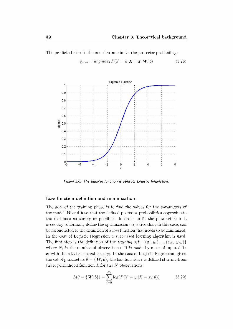
32 Chapter 3. Theoretical background
The predicted class is the one that maximize the posterior probability:
ypred = argmaxkP (Y = k|X = x;W, b) (3.28)
Figure 3.6: The sigmoid function is used for Logistic Regression.
Loss function denition and minimization
The goal of the training phase is to nd the values for the parameters of
the model W and b so that the dened posterior probabilities approximate
the real ones as closely as possible. In order to t the parameters it is
necessary to formally dene the optimization objective that, in this case, can
be reconducted to the denition of a loss function that needs to be minimized.
In the case of Logistic Regression a supervised learning algorithm is used.
The rst step is the denition of the training set : (x1, y1), ..., (xNs , yNs)where Ns is the number of observations. It is made by a set of input data
xi with the relative correct class yi. In the case of Logistic Regression, given
the set of parameters θ = W, b, the loss function l is dened starting from
the log-likelihood function L for the N observations:
L(θ = W, b) =
Ns∑i=0
log(P (Y = yi|X = xi; θ)) (3.29)

3.3. Classication methods 33
and
loss(θ) = −L(X; θ). (3.30)
The explicit computation (i.e. a close form solution) of the minimum of a
generic, non-quadratic, function it is not possible. It this case the minimum,
that, however, could be a local minimum, must be found by means of itera-
tive numerical methods. In the literature there are several approaches that
can be adopted in order to minimize the loss function. A simple though
eective iterative method is called Stochastic Gradient Descent (SGD). The
idea behind the SGD approach is that a minimum of the function can be
found iteratively updating the parameters of the model by moving toward
the negative gradient direction with a constant step. A simple graphical
example is shown in gure 3.7.
θ
loss(θ)
Local minimum
Starting point
Global minimum
Convergence
Figure 3.7: The gure shows a simple 2-dimensional example of application of SGD.
Starting from a random initialization of the parameters their value is updated moving
towards the direction specied by the gradient of the loss function. The random initial-
ization can result in a local minimum convergence. For probabilistic models, however, it
is not desirable to end in a global minimum since in that case there would be overtting
of the training distribution.
More formally, after a rst, generically random, initialization of the pa-
rameters, the update rule for their value is:
θk+1 ← θk − ρ∂loss(θ)∂θ
(3.31)
Where k indicates the iteration number, ρ is the incremental step also called
learning rate. After a number of steps, the parameters found at the end of
34 Chapter 3. Theoretical background
the process should converge to a minimum of the loss function. Even if this
method is simple and eective it still suers from a number of problems:
• if the classes are not separable, the convergence of this algorithm is
not guaranteed;
• the choice of the learning rate is crucial: if it is chosen to be too large
the algorithm does not converge. If it is chosen to be too small, on the
other hand, the convergence, if possible, may require a lot of time;
• it requires the computation of the gradient of the loss function that can
be a dicult task and can suer from numerical stability problems.
3.3.2 One-Hidden Layer Multi-Layer Perceptron Neural Net-
work
The Multi-Layer Perceptron Neural Network (MLPNN) is a non-linear dis-
criminative classier where the input is rst transformed using a learnt trans-
formation Θ. Through the transformation Θ, the input data are projected
into a space where it becomes linearly separable. Afterwards, on the trans-
formed data a linear classier is applied. Usually, Logistic Regression is used
as classier.
The MLPNN can be seen as a computational acyclic graph where the
outputs of the node at every layer are given as inputs of the node in the
following one. Every node can be seen as a computing unit capable of eval-
uating a single primitive function of its input [35]. An MLPNN can have an
arbitrary number of layers, in the case of one-hidden layer there are:
• an input layer, that has a number of elements equal to the dimensions
of a generic observation of the input dataset. The nodes in this layer
have no predecessors;
• a single hidden layer, with an arbitrary number of elements;
• an output layer, that has a number of elements equal to the number of
possible classes of the classication problem. The nodes in this layer
have no successors.
Formally, a one-hidden layer MLPNN can be modeled as a function f :
RM → RK , withM representing the size of an input observation x and K is
3.3. Classication methods 35
the number of classes. The function f(x) in matrix notation can be written
as:
f(x) = g(b(2) +W (2)(s(b(1) +W (1)x))). (3.32)
b(1) and b(2) are the bias vectors for the rst and second layer, W (1) and
W (2) are the weight matrices. g(z) and s(x) are called activation functions.
The function s(x) is typically chosen to be tanh(x) = (ex − e−x)/(ex + e−x)
or sigmoid(x) = 1/(1 + e−x) and are applied to vectors separately on each
element. The function f(x) is made by:
• the hidden layer vector: h(x) = Θ(x) = s(b(1) +W (1)x). The choice of
s(x) corresponds to the choice of the non-linear transformation in the
process;
• the output layer: o(x) = g(b(2) +W (2)Θ(x)) corresponds to multi-class
Logistic Regression of the transformed dataset.
The training process of a MLPNN is done in a supervised manner. Similarly
to the Logistic Regression approach, the training process iteratively adjusts
the parameters with the goal of minimizing a Loss Function. As the Logistic
Regression case, the Loss Function is chosen to be the negative log-likelihood
(eq. 3.30). The minimization process is done, with the same approach as
before, using SGD. This time, however, since the network is composed by
dierent layers the gradient computation must be applied recursively. This
can be done, thanks to the graph structure of the network, using the chain
rule for derivatives, that species how the partial derivative for a node can be
obtained recursively from the partial derivatives for his parents [18]. Thanks
to this, the updates of the SGD for a MLPNN can be found by means of a
two-pass training stage:
• in the forward step an observation is fed to the network and the pre-
diction values are computed based on the current state of the weights;
• in the backward step the errors of the output layer are computed and
then back-propagated through the network. All the sets of errors are
used to compute the gradients for the SGD update rules.
In order to prevent overtting of the training distribution, the Loss Function
is modied and a regularization term is often added. This has the eect of
penalizing large values of the parameters. The function then becomes
R(θ) = loss(θ) + λJ(θ) (3.33)

36 Chapter 3. Theoretical background
where
J(θ) =
|θ|∑j=0
|θj |p 1
p
. (3.34)
Typically p = 2 and, in this case, the regularizer is called weight decay.
…
…
…
Input Layer
Output Layer
Hidden Layer
h1
h2
hH-1
hH
y1
yK-1
yK
x1
x2
xM
Figure 3.8: The graphical representation of a one hidden layer multilayer perceptron
with M input units, H hidden units and K output units
3.3.3 Deep Belief Networks
Deep Learning algorithms have been inspired by recent discovery in the study
of human brain. Scientists in this eld that deals with the understanding
of the neocortex, which is associated to many cognitive abilities, discovered
that it works in a hierarchical fashion. The input signal, in our brain, is
not explicitly pre-processed but it propagates through a complex hierarchy
of modules that learn to represent observation based on the regularity they
exhibit [1]. Human being, thus, is able to decompose a problem into sub-
problems every time with a higher level of abstraction. This process is what
deep learning algorithms are designed to mimic.
The input of a learning system can be generally seen as a high dimen-
sional entity, where the observed variables are related by unknown complex

3.3. Classication methods 37
statistical relationships called factors of variations [5]. The goal of deep
architectures is to try to overcome the problem of the lack of an a priori
analytical knowledge of these factors. Ideally a deep network could be able
to automatically discover the important aspects of a distribution through
dierent level of abstractions, similarly to the behavior of the human brain.
This is done creating feature hierarchies where higher level features are the
result of a composition of the lower level ones.
The kind of deep learning networks that we use in this thesis are the Deep
Belief Networks (DBNs). They have been introduced by Hinton and his team
in [21], where he solved the problem of the training of the multi-hidden layer
neural networks proposing a greedy algorithm that trains one layer at the
time in a unsupervised manner. This is possible because they are dened as
probabilistic generative models made by several layers of Restricted Boltz-
mann Machines (RBMs). As mentioned before, generative models, in con-
trast with the discriminative models such as the standard neural networks,
are able to provide a joint probability distribution over labels and observ-
able data. They are, thus, able to estimate both P (Label|Observation) and
P (Observation|Label), while discriminative models are limited just to the
estimation of the former P (Obsevation|Label).Since DBNs are based on Restricted Boltzmann Machines that are a par-
ticular case of Energy Based Models, in the following subsections we will
review the theoretical concepts behind these models and then we will ex-
plain the training algorithm for a Deep Belief Network.
Energy based models
Energy based probabilistic models dene a probability distribution using
the concept of energy function. The main idea behind these models, is to
associate a scalar energy to each conguration of the variables of interest [5].
The learning process has the goal of modify that energy function in a way
that its shape has particular properties. For example, it can be desirable
that plausible congurations have low energy. The probability distribution
of a variable x can be formally dened as:
P (x) =e−Energy(x)
Z, (3.35)
where Z is called partition function and it is a normalizing factor dened as:
Z =∑x
e−Energy(x). (3.36)
38 Chapter 3. Theoretical background
The energy function has been reformulated by Hinton [19], in the product of
experts formulation, as a sum of terms:
Energy(x) =∑i
fi(x), (3.37)
in this way the probability becomes:
P (x) ∝∏i
Pi(x) ∝∏i
e−fi(x). (3.38)
Each expert Pi(x) enforces constraints on x and, in this way, it can be
seen as a detector of implausible congurations of x. The advantage of this
formulation is that the energy forms a distributed representation partitioning
the space according to all the possible congurations, where each expert can
have its constraint violated or not. In order to increase the expressive power
of the model, hidden variables, that are not directly observed variables, are
introduced. In this way x becomes the visible part and h the hidden part
where:
P (x, h) =e−Energy(x,h)
Z. (3.39)
This equation can be rewritten introducing the concept of free energy :
FreeEnergy(x) = − log∑h
e−Energy(x,h), (3.40)
using this notation, the expression of the marginal probability P (x) becomes
similar to the initial formulation:
P (x) =e−FreeEnergy(x)
Z(3.41)
with Z =∑
x FreeEnergy(x). The use of the free energy notation allows to
derive a simple expression for the computation of the log-likelihood gradient:
EP
[∂ logP (x)
∂θ
]= −EP
[∂FreeEnergy(x)
∂θ
]+ EP
[∂FreeEnergy(x)
∂θ
](3.42)
where E are expectations over x, P the training set empirical distribution
and P the model's distribution. If it is possible to sample from P and to ob-
tain a simple computational expression for the free energy, then a stochastic
estimator of the log-likelihood gradient can be found using Markov Chain
Monte-Carlo (MCMC) method [4]. In the next subsection, we will see that
the Restricted Boltzmann Machines allow to have a simple expression of the
free energy and, with a few assumptions, an eective training method can
be obtained.

3.3. Classication methods 39
Restricted Boltzmann Machines
The Restricted Boltzmann Machine (RBM) is an energy based model with
the presence of a visible layer x and a hidden layer h. The convenient prop-
erty of this kind of model is that hidden nodes hi are independent from each
other when conditioning on x and vice-versa. This fact can be seen rep-
resenting the RBM with a undirected graph (gure ...) where there are no
connections between elements belonging to the same layer. The RBM can be
thought as two sets of basis vectors, one which reduces the dimensionality of
the data and the other that reconstructs it [37]. Formally, the RBM energy
function can be expressed as:
Energy(x, h) = −b′x− c′h− h′Wx (3.43)
where W is the weight matrix and b and c are the biases associated respec-
tively to the input and the hidden units. The free energy of an RBM can be
computed eciently as:
FreeEnergy(x) = −b′x−∑i
log∑hi
ehi(ci+Wix). (3.44)
The main advantage of using the RBM is that, due to the lack of connections
between elements of the same layer, the conditional probabilities P (h|x) and
P (x|h) can be factorized as:
P (h|x) =∏i
P (hi|x) (3.45)
and
P (x|h) =∏i
P (xi|h). (3.46)
In the most common case, the hidden variable is binomial, i.e. hi ∈ 0, 1, ∀i.In this case, the expression of P (hi = 1|x) becomes the equation of a neuron
of a neural network with sigmoidal activation function:
P (hi = 1|x) =eci+Wix
1 + eci+Wix= sigm(ci +Wix). (3.47)
If the visible layer is binomial too, the same derivation can be done for
P (xi = 1|h):
P (xi = 1|h) = sigm(bj +W ′jh) (3.48)
The training of an RBM can be done in an ecient way using the al-
gorithm of Contrastive Divergence (CD-1) by found by Hinton [21]. In his
formulation, two approximations in the model are done:
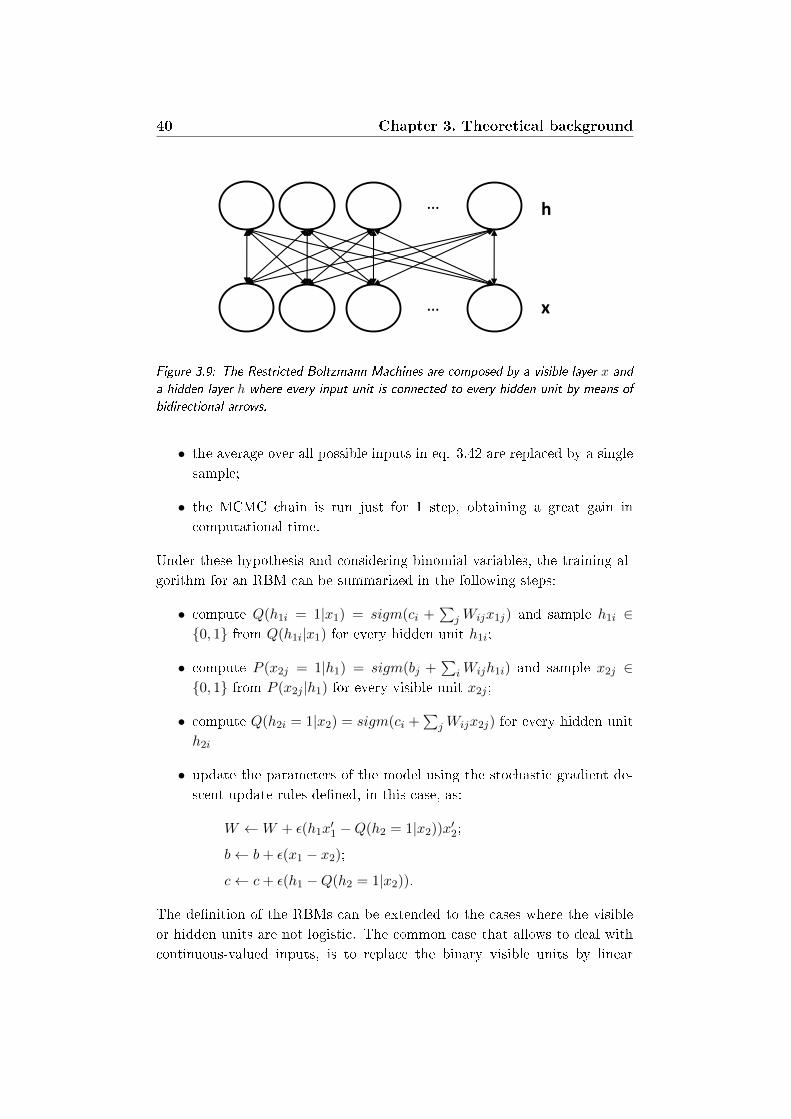
40 Chapter 3. Theoretical background
…
… x
h
Figure 3.9: The Restricted Boltzmann Machines are composed by a visible layer x and
a hidden layer h where every input unit is connected to every hidden unit by means of
bidirectional arrows.
• the average over all possible inputs in eq. 3.42 are replaced by a single
sample;
• the MCMC chain is run just for 1 step, obtaining a great gain in
computational time.
Under these hypothesis and considering binomial variables, the training al-
gorithm for an RBM can be summarized in the following steps:
• compute Q(h1i = 1|x1) = sigm(ci +∑
jWijx1j) and sample h1i ∈0, 1 from Q(h1i|x1) for every hidden unit h1i;
• compute P (x2j = 1|h1) = sigm(bj +∑
iWijh1i) and sample x2j ∈0, 1 from P (x2j |h1) for every visible unit x2j ;
• compute Q(h2i = 1|x2) = sigm(ci +∑
jWijx2j) for every hidden unit
h2i
• update the parameters of the model using the stochastic gradient de-
scent update rules dened, in this case, as:
W ←W + ε(h1x′1 −Q(h2 = 1|x2))x′2;
b← b+ ε(x1 − x2);
c← c+ ε(h1 −Q(h2 = 1|x2)).
The denition of the RBMs can be extended to the cases where the visible
or hidden units are not logistic. The common case that allows to deal with
continuous-valued inputs, is to replace the binary visible units by linear

3.3. Classication methods 41
units with independent Gaussian noise [20]. In this case, the energy function
becomes:
Energy(x, h) =∑i
(vi − bi)2
2σ2i− c′h−
∑i,j
viσihjwij (3.49)
where σi is the standard deviation of the Gaussian noise for the visible unit
i. In order to avoid the learning of the variance of the noise using CD-1,
that is a dicult task, a normalization of the input data can be applied.
In particular, they are normalized to have zero mean and unit variance. In
this case, it is possible to set the value of σ in eq. 3.49 equal to 1. With
this formulation, the reconstructed value of the visible unit in the second
step of the training algorithm is equal to his top-down input plus his bias:
x2j =∑
iWijh1i + bj .
Formulation and training of a DBN
A DBN with n layers is able to model the joint distribution between an
observed vector x and n hidden layers as:
P (x, h(1), ..., h(n)) =
(n−2∏k=0
P (h(k)|h(k+1))
)P (h(k−1), h(k)). (3.50)
With this formulation x = h(0), P (h(k−1)|h(k)) is the visible-given-hidden
conditional distribution of an RBM at layer k of the DBN, while P (h(k−1), h(k))
is the joint distribution of the top layer RBM as shown in gure 3.10.
The denition of the DBN as a generative model using RBM allowed Hin-
ton [21] to derive a training strategy that overcomes the traditional problems
concerning the training of Multi Layer Perceptron Neural Networks. Starting
from random initialization, in fact, deep Neural Networks performed worse
than shallow architectures with 1 or 2 hidden layers [5]. This is due to the fact
that standard gradient descent approach with random initialization is unable
to optimally tune the parameters of the lower layers of the network [5]. This
fact can hurt rather than help the top two layers to perform classication
with a good generalization. Hinton introduced an unsupervised pre-training
phase that showed a great improvement in the classication error with re-
spect to the random initialization of the parameters [21]. The idea behind
this algorithm is that a complicated model can be learnt combining a set of
simpler models learned sequentially. This greedy approach rst trains the
lower layer with an unsupervised learning algorithm, then the output of the
rst layer is used as input for the unsupervised learning of the following layer.
The process is repeated for every layer in the network. One of the reasons

why this approach works is that the injection of unsupervised training signal
at each layer can guide the parameters of that layer toward better regions in
the parameter space (i.e. close to solutions capturing signicant statistical
structure of the data). The importance of doing a pre-training phase rely
also in the fact that with this approach a better tuning of the lower layers
of the network can be obtained. Unsupervised pre-training, thus, acts like a
data dependent regularized [5].
One epoch of the greedy pre-training algorithm proposed by Hinton, can
be summarized in the following steps. First, all the parameters, weights and
biases, of each layer of the network are randomly initialized. Then, they are
updated as follows:
• the rst layer is trained as an RBM with Contrastive Divergence using
the input vector x as the visible layer of the model x = h(0);
• the hidden layer of the rst RBM is used to obtain a representation
(i.e. the mean activations or directly the samples) of the input of the
RBM at the following layer;
• train the second layer RBM using the chosen data from the previous
layer as training examples for the visible layer of this RBM;
• repeat the second and third step for every layer in the network propa-
gating upward the samples or mean activation values.
All these four steps are, then, repeated for the desired number of epochs.
After the DBN has been initialized by pre-training, a supervised ne-
tuning phase is performed. The network is, then, treated like a normal
Multi Layer Perceptron Neural Network (gure 3.11) and the optimization
of the parameters is done in the standard way using Stochastic Gradient
Descent with back-propagation.
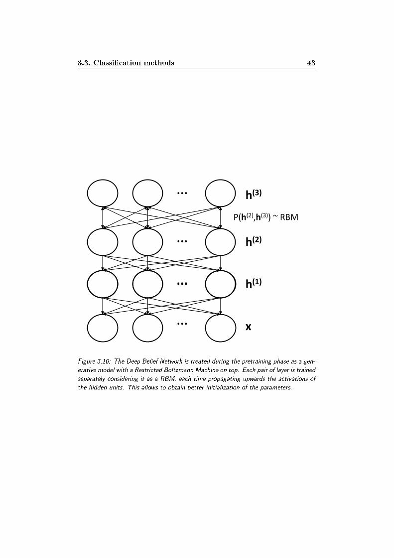
3.3. Classication methods 43
…
… x
h(1)
h(2)
h(3)
…
…
…
P(h(2),h(3)) ~ RBM
Figure 3.10: The Deep Belief Network is treated during the pretraining phase as a gen-
erative model with a Restricted Boltzmann Machine on top. Each pair of layer is trained
separately considering it as a RBM, each time propagating upwards the activations of
the hidden units. This allows to obtain better initialization of the parameters.

44 Chapter 3. Theoretical background
…
… x
h1
h2
h3
y
…
…
…
…
Figure 3.11: During the netuning and classication phases, the Deep Belief Network
is treated like a Multi Layer Neural Network, a discriminative model. The netuning
is done using Stockastic Gradient Descent with backpropagation of the errors, the
classication is simply done by means of a forward pass of the network.
Chapter 4
System overview
This chapter is dedicated to the description of our approach to the chord
classication problem.
The overall process is composed by various steps that together can be
grouped in two main phases, as summarized in Figure 4.1. The rst phase
regards the extraction of the chromagram from the audio signal and will be
addressed in section 4.1. In our work we compared two main methods for
the chromagram computation that will be described in section 4.1.2. The
chromagram extraction involves also a denoising process. In this study we
compared four type of lters, introducing two lters that has never been
tested, that will be described in section 4.1.3 as well as how we applied them
to denoise the chromagram.
The second phase regards the classication procedure. Once the chroma-
gram has been computed in the feature extraction process, each frame, or
chroma vector, is analyzed and classied associating it to a chord label. The
novel methods we propose in this study for the classication procedure are
based on machine learning techniques. The various phases and the descrip-
tion of their application to the chord classication problem will be addressed
in section 4.2. In particular, we used three types of classiers: Logistic
Regression, One Hidden Layer Multilayer Perceptron and Deep Belief Net-
works. In this way we wanted to explore if and how the use of non linear
classiers and deep learning techniques can bring a gain in the performances
with respect to the linear classier and state-of-the art template matching
approaches. Using machine learning approaches, the quality of the obtained
transcription is no more dependent by the hand-made creation of chords
templates dierently from template based approaches (section 4.3). In fact,
we used them to directly classify chroma vectors using each chroma vector
as input observations to the probabilistic classiers. However, in order to
45

46 Chapter 4. System overview
perform the classication these methods require a training process.
In this chapter we will also address a variation of the template-matching
method proposed by [32] that will be described in section 4.3. The procedure
followed by this approach involves the comparison of each chroma vector with
a set of previously created chords templates using a measure of similarity.
Dierently from the approach in [32], we performed temporal ltering after
the classication has been done instead of lter the matrix of distances and
the created chords templates are used not normalized.
4.1 Feature extraction
In this section we will present the feature extraction phase of the system.
First we will give a general description of the entire process, with a review of
all the phases involved and the dierences between the type of chromagrams
that we compared. At the end we will present the denoising process with a
description of the lters that we used.
4.1.1 General description
As we mentioned in Chapter 3, the goal of the feature extraction phase is
to extract a meaningful feature from the audio signal that can be used to
perform automatic chord classication. In order to select the best feature in
terms of classication performance, we tested dierent procedures starting
from the same standard baseline described in section 3.2. The main compu-
tational blocks involved in this process and the dierent alternatives that we
tested are shown in Figure 4.2.
The standard baseline involves three main steps. The rst step of the
process aims to obtain a frequency versus time representation of the audio
signal. This is done computing the Short Time Fourier Transform (STFT)
Xstft(k, r) of the input signal and subsequently use the Constant-Q Trans-
form (CQT) to obtain a spectrum with log-frequency resolution Xcq(k, r)
instead of the linearly spaced representation given by the STFT. For clarity,
these two steps can be grouped in an overall step whose goal is the computa-
tion of the log-spectrum of the input signal. After the frequency versus time
representation Xcq(k, r) has been calculated, the successive step is to obtain
a pitch-class versus time representation of the input signal. This overall step
contains two smaller steps. In the rst one, the sum of the contribution in
terms of energy of each pitch class in the total number of octaves considered
by the CQT is performed. The result is a 36 bins versus time representation
of the input signal C36(b, r). After this process, the chromagram is tuned.

4.1. Feature extraction 47
Feature
Extraction
Classification
x(n)
Cβ(k,r)
l(r)
Figure 4.1: The chord transcription process involves two main phases. A feature ex-
traction phase where the chromagram is extracted from the audio signal and processed.
The subscript β indicates the number of bins of the chromagram that, in our case,
will be of 12 or 36 depending on the classication method used. The second phase is
the classication phase, where the chromagram is used as a feature to compute the
classication obtaining a chord label vector.

48 Chapter 4. System overview
Finally, the last step is to reduce the number of bins to 12 summing the val-
ues of the 36 bins representation within every semitone obtaining C12(b, r).
For the detailed description of these phases and the notation we remind to
Section 3.2.3. This is the rst method that we used as standard baseline.
The two other alternatives that we tested are, in fact, two variations of the
previously summarized baseline and they have been proposed in [29].
The rst alternative involves the introduction of a post processing phase
of the log-spectrum that makes use of the A-Weighting of Xcq(k, r). The
description of this processing step will be done in Section 4.1.2. The baseline
of this feature extraction approach involves four steps. The rst step is the
same of the standard baseline that is the computation of the log-spectrum
by means of the Constant-Q transform. After this step, the A-Weighting is
applied to the resulting representation. The last two steps are the same of
the standard baseline.
The second alternative makes use of the Harmonic Percussive Signal Sep-
aration algorithm addressed in Section 3.2.2. In particular, it can be sum-
marized in four processing steps. The rst step is the extraction of the
harmonic components of the input audio signal xh(n) as described in Sec-
tion 3.2.2. This time, the computation of the log-spectrum is not done on
the input signal, it is done instead starting from the harmonic components
extracted by means of the HPSS algorithm. The other three steps of the
process are the same of the standard baseline.
The pitch class versus time representations of the audio signal obtained
by means of these three techniques are very noisy and do not allow to have
a good transcription of the chords of a song, as we will see in chapter 5. For
this reason it is necessary to introduce a ltering stage where a time domain
lter is applied to the chromagram. In our work we tested how the chord
classication rate changes with respect to the application of four dierent
types of lters. They are the averaging lter, the median lter and two
lters that have never been tested for this purpose that are the geometric
mean lter and the harmonic mean lter. We also tested how the perfor-
mance change if they are applied before the last step in the chromagram
computational baseline or at the end of the process as last operation. The
summarization of the dierent phases can be found in Figure 4.2.
In the following sections we will address the A-Weighting block and the
ltering stage respectively in Section 4.1.2 and Section 4.1.3, the other com-
putational block have been addressed in Section in 3.2.
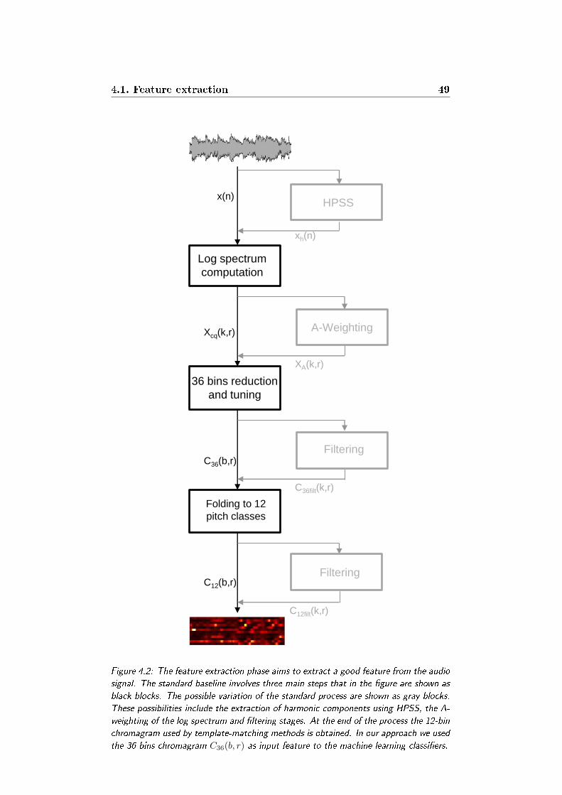
4.1. Feature extraction 49
HPSS
Log spectrum
computation
36 bins reduction
and tuning
Folding to 12
pitch classes
A-Weighting
Filtering
Filtering
x(n)
xh(n)
Xcq(k,r)
XA(k,r)
C36(b,r)
C36filt(k,r)
C12filt(k,r)
C12(b,r)
Figure 4.2: The feature extraction phase aims to extract a good feature from the audio
signal. The standard baseline involves three main steps that in the gure are shown as
black blocks. The possible variation of the standard process are shown as gray blocks.
These possibilities include the extraction of harmonic components using HPSS, the A-
weighting of the log spectrum and ltering stages. At the end of the process the 12-bin
chromagram used by template-matching methods is obtained. In our approach we used
the 36 bins chromagram C36(b, r) as input feature to the machine learning classiers.
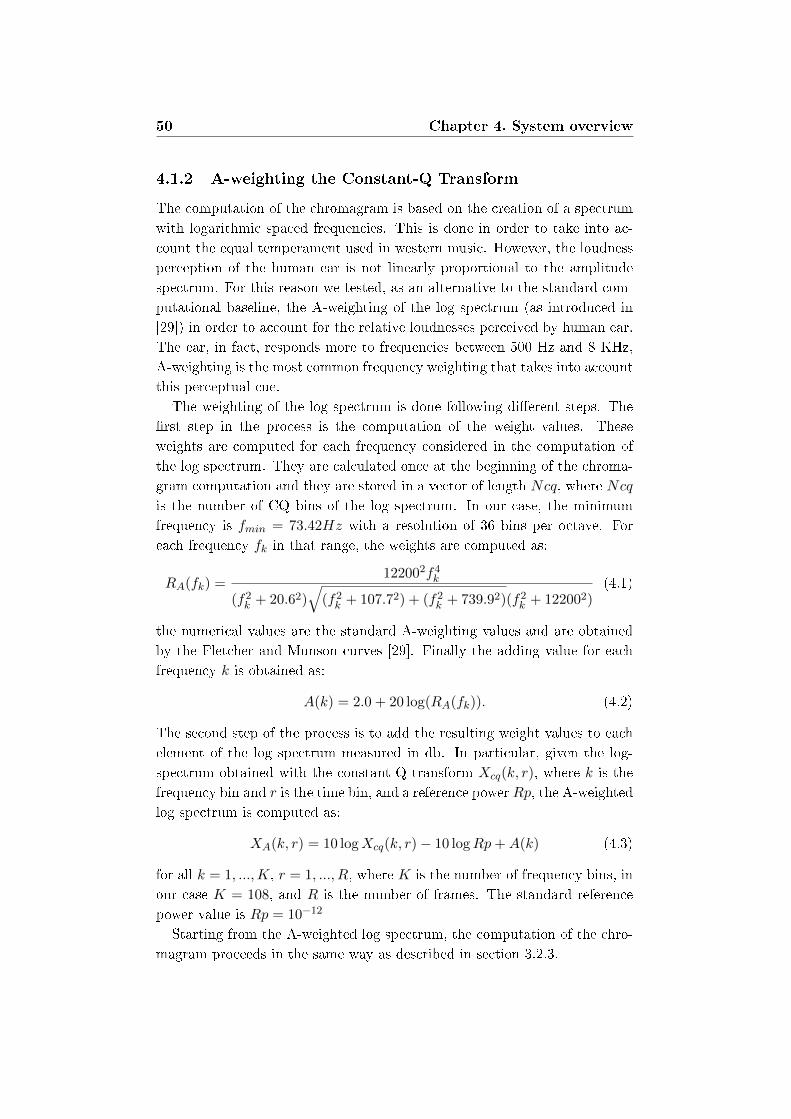
50 Chapter 4. System overview
4.1.2 A-weighting the Constant-Q Transform
The computation of the chromagram is based on the creation of a spectrum
with logarithmic spaced frequencies. This is done in order to take into ac-
count the equal temperament used in western music. However, the loudness
perception of the human ear is not linearly proportional to the amplitude
spectrum. For this reason we tested, as an alternative to the standard com-
putational baseline, the A-weighting of the log spectrum (as introduced in
[29]) in order to account for the relative loudnesses perceived by human ear.
The ear, in fact, responds more to frequencies between 500 Hz and 8 KHz,
A-weighting is the most common frequency weighting that takes into account
this perceptual cue.
The weighting of the log spectrum is done following dierent steps. The
rst step in the process is the computation of the weight values. These
weights are computed for each frequency considered in the computation of
the log spectrum. They are calculated once at the beginning of the chroma-
gram computation and they are stored in a vector of length Ncq, where Ncq
is the number of CQ bins of the log spectrum. In our case, the minimum
frequency is fmin = 73.42Hz with a resolution of 36 bins per octave. For
each frequency fk in that range, the weights are computed as:
RA(fk) =122002f4k
(f2k + 20.62)√
(f2k + 107.72) + (f2k + 739.92)(f2k + 122002)(4.1)
the numerical values are the standard A-weighting values and are obtained
by the Fletcher and Munson curves [29]. Finally the adding value for each
frequency k is obtained as:
A(k) = 2.0 + 20 log(RA(fk)). (4.2)
The second step of the process is to add the resulting weight values to each
element of the log spectrum measured in db. In particular, given the log-
spectrum obtained with the constant-Q transform Xcq(k, r), where k is the
frequency bin and r is the time bin, and a reference power Rp, the A-weighted
log spectrum is computed as:
XA(k, r) = 10 logXcq(k, r)− 10 logRp+A(k) (4.3)
for all k = 1, ...,K, r = 1, ..., R, where K is the number of frequency bins, in
our case K = 108, and R is the number of frames. The standard reference
power value is Rp = 10−12
Starting from the A-weighted log spectrum, the computation of the chro-
magram proceeds in the same way as described in section 3.2.3.
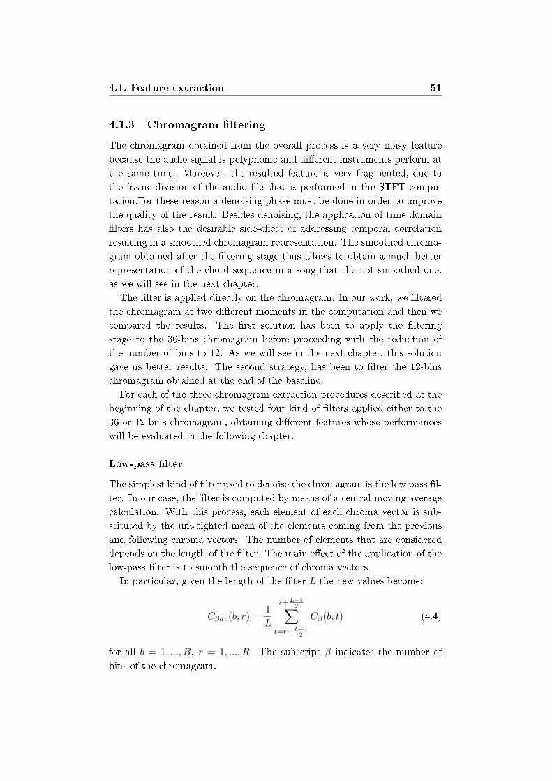
4.1. Feature extraction 51
4.1.3 Chromagram ltering
The chromagram obtained from the overall process is a very noisy feature
because the audio signal is polyphonic and dierent instruments perform at
the same time. Moreover, the resulted feature is very fragmented, due to
the frame division of the audio le that is performed in the STFT compu-
tation.For these reason a denoising phase must be done in order to improve
the quality of the result. Besides denoising, the application of time domain
lters has also the desirable side-eect of addressing temporal correlation
resulting in a smoothed chromagram representation. The smoothed chroma-
gram obtained after the ltering stage thus allows to obtain a much better
representation of the chord sequence in a song that the not smoothed one,
as we will see in the next chapter.
The lter is applied directly on the chromagram. In our work, we ltered
the chromagram at two dierent moments in the computation and then we
compared the results. The rst solution has been to apply the ltering
stage to the 36-bins chromagram before proceeding with the reduction of
the number of bins to 12. As we will see in the next chapter, this solution
gave us better results. The second strategy, has been to lter the 12-bins
chromagram obtained at the end of the baseline.
For each of the three chromagram extraction procedures described at the
beginning of the chapter, we tested four kind of lters applied either to the
36 or 12 bins chromagram, obtaining dierent features whose performances
will be evaluated in the following chapter.
Low-pass lter
The simplest kind of lter used to denoise the chromagram is the low pass l-
ter. In our case, the lter is computed by means of a central moving average
calculation. With this process, each element of each chroma vector is sub-
stituted by the unweighted mean of the elements coming from the previous
and following chroma vectors. The number of elements that are considered
depends on the length of the lter. The main eect of the application of the
low-pass lter is to smooth the sequence of chroma vectors.
In particular, given the length of the lter L the new values become:
Cβav(b, r) =1
L
r+L−12∑
t=r−L−12
Cβ(b, t) (4.4)
for all b = 1, ..., B, r = 1, ..., R. The subscript β indicates the number of
bins of the chromagram.
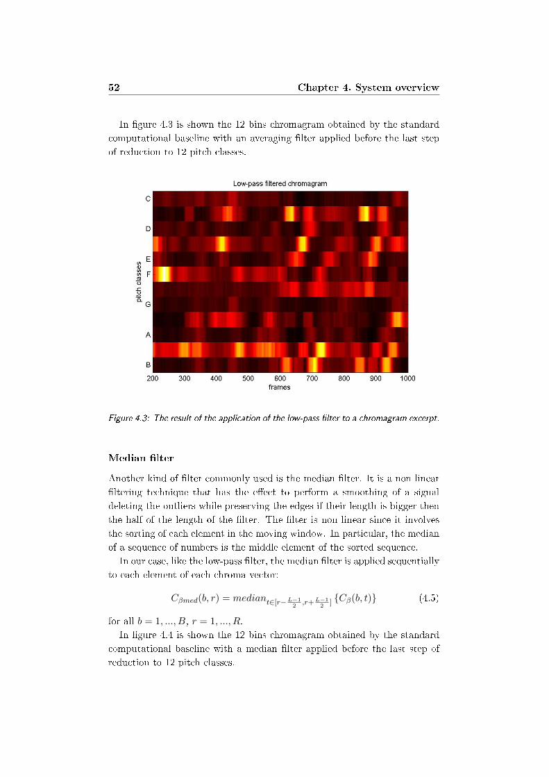
52 Chapter 4. System overview
In gure 4.3 is shown the 12 bins chromagram obtained by the standard
computational baseline with an averaging lter applied before the last step
of reduction to 12 pitch classes.
Figure 4.3: The result of the application of the low-pass lter to a chromagram excerpt.
Median lter
Another kind of lter commonly used is the median lter. It is a non linear
ltering technique that has the eect to perform a smoothing of a signal
deleting the outliers while preserving the edges if their length is bigger then
the half of the length of the lter. The lter is non linear since it involves
the sorting of each element in the moving window. In particular, the median
of a sequence of numbers is the middle element of the sorted sequence.
In our case, like the low-pass lter, the median lter is applied sequentially
to each element of each chroma vector:
Cβmed(b, r) = mediant∈[r−L−12,r+L−1
2] Cβ(b, t) (4.5)
for all b = 1, ..., B, r = 1, ..., R.
In gure 4.4 is shown the 12 bins chromagram obtained by the standard
computational baseline with a median lter applied before the last step of
reduction to 12 pitch classes.
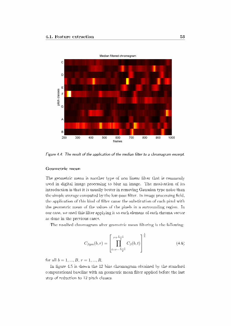
4.1. Feature extraction 53
Figure 4.4: The result of the application of the median lter to a chromagram excerpt.
Geometric mean
The geometric mean is another type of non linear lter that is commonly
used in digital image processing to blur an image. The motivation of its
introduction is that it is usually better in removing Gaussian type noise than
the simple average computed by the low-pass lter. In image processing eld,
the application of this kind of lter cause the substitution of each pixel with
the geometric mean of the values of the pixels in a surrounding region. In
our case, we used this lter applying it to each element of each chroma vector
as done in the previous cases.
The resulted chromagram after geometric mean ltering is the following:
Cβgm(b, r) =
r+L−12∏
t=r−L−12
Cβ(b, t)
1L
(4.6)
for all b = 1, ..., B, r = 1, ..., R.
In gure 4.5 is shown the 12 bins chromagram obtained by the standard
computational baseline with an geometric mean lter applied before the last
step of reduction to 12 pitch classes.

54 Chapter 4. System overview
Figure 4.5: The result of the application of the geometric mean lter to a chromagram
excerpt.
Harmonic mean
The harmonic mean lter is the last lter that we tried. Like geometric mean
is a commonly used lter in image processing in order to remove Gaussian
noise. Together with arithmetic mean and geometric mean, it is part of the
family of Pythagorean mean lters. The application to chromagram noise
reduction is the same as the three previous lters since each element of each
chroma vector is replaced with the harmonic mean of the elements of the
surrounding vectors.
The new chroma vector is thus computed as:
Cβhm(b, r) =L∑r+L−1
2
t=r−L−12
1Cβ(b,r)
(4.7)
for all b = 1, ..., B, r = 1, ..., R.
In gure 4.6 is shown the 12 bins chromagram obtained by the standard
computational baseline with an harmonic mean lter applied before the last
step of reduction to 12 pitch classes.

4.2. Machine learning classication 55
Figure 4.6: The result of the application of the harmonic mean lter to a chromagram
excerpt.
4.2 Machine learning classication
In our work, we decided to approach the Automatic Chord Recognition prob-
lem with a change of perspective with respect to the template matching based
approach. This change lies in the fact that we decided to overcome the prob-
lems of the creation of a model of templates of chroma vectors and of the
choice of a correct measure of distance.
Instead of creating a model of chord templates followed by the compu-
tation of a similarity measure, we used machine learning classication algo-
rithms that have been trained to automatically recognize chords from chroma
vectors. Our method can be, thus, seen as a blind classication approach
where no other information, except for the correct label associated to a
chroma vector needed for the training stage, is used to compute the classi-
cation. The goal of our work has been to understand if this kind of approach
can improve the chord recognition accuracy with respect to the template
matching based methods.
Theoretically, the main advantage of this approach is that the use of Neu-
ral Networks and Deep Belief Networks allows to better learn the contribu-
tion of each feature of the input data to the output class even in presence

56 Chapter 4. System overview
of noise. These kind of non-linear classiers, in fact, are designed to model
complex non linear functions that link input observations to output classes
by means of one or more layer of non linear transformations of the input
observations. In our case they are trained to learn a probabilistic model that
allows to identify the most probable chord associated to each chroma vector.
However, the accuracy of the model learnt by machine learning classiers
and, in particular, by the Multilayer Perceptron and Deep Belief Networks
depends on a variety of factors of dicult interpretation.
To simplify the learning process and reduce the error probability, the chord
recognition is limited to major and minor chords. Other complex chords like
augmented or dimished chords, dominant and maj7 are considered parts of
those two main categories. This is usually done in chord recognition systems
since complex chords unlikely occur in pop music [16].
Our classication algorithm is divided in dierent phases that are sum-
marized in Figure 4.7. Each chroma vector represents an input observation
of the classier. In particular, we used as input feature the high resolution
chromagram obtained by the feature extraction phase before the reduction
of the pitch class axis to 12. Each input observation of the classier thus
will be a row vector of 36 elements.
Each element of an observation, that in the chromagram corresponds to a
pitch class bin, is interpreted by the machine learning classier as the value
of a feature of the input observation. The rst step in the computation is to
normalize the values of these features such that they fall in the same range.
This is done because the performances of the training algorithm is inuenced
by the dynamic range of the features. These arguments will be addressed in
section 4.2.1.
The step that usually follows feature normalization before the training
process is the whitening. It is a processing feature space in order to ensure
linear independence of the features. In our case, this step is not necessary
since the features are already linearly independent. So, once the normal-
ization has been done, a training and evaluation sets are created starting
from a dataset of chroma vectors and the classier is trained in a supervised
manner. The training and evaluation sets have been previously labelled as
required by the supervised training algorithms. The Deep Belief Networks
have also been pre-trained in an unsupervised manner before the supervised
procedure, but this has only been possible for specic normalizations of the
input observations as we will see in Section 4.2.1.
The parameters of the best model are then loaded and the learnt model is
used to compute the classication of new unseen chroma vectors. The classi-
ers have been trained to recognize just major and minor chords. The recog-

4.2. Machine learning classication 57
nition of the no-chord chroma vectors is done in a successive step analyzing
each frame. At the end, the resulting classication vector is post-processed
using a temporal domain lter that has the dual eect of addressing temporal
correlation and of eliminating the outliers.
Summarizing, the dierent steps of the algorithm can be listed as follow-
ing:
• normalization of the input features or feature scaling ;
• learning a probabilistic model using a supervised approach considering
a training and evaluation set of chroma vectors;
• classication of new unseen songs using the best learnt model during
the training stage;
• no-chord recognition and addressing temporal correlation using tem-
poral domain lter.
All these phases will be addressed in the following sections.
4.2.1 Feature Scaling
The rst step in our machine learning classication algorithm is the normal-
ization of each feature of every input observation in order to map their values
in the same range. This process is called feature scaling and is done for ev-
ery chromagram that will compose the training, evaluation and classication
sets.
This pre-processing step is commonly done when dealing with machine
learning classication algorithms because it can speed up the process of
minimization of the cost function. In our case, in particular, it is neces-
sary because the algorithm that we used, Stochastic Gradient Descent, it is
known to be highly sensitive to feature scaling. The activation functions of
the classiers also are sensitive to the range of the values of the input ob-
servations. If the range is too small, in fact, the activation functions (gure
3.6) mainly work in the linear region reducing the discriminative power of
the model.
Another important reason for doing feature scaling is that the pre-training
algorithms of the Deep Belief Network work only if the input distribution
have precise characteristics. The unsupervised learning algorithm, in fact,
aims to learn important characteristics of the input distribution, but the
Restricted Boltzmann Machines makes assumptions on the nature of the
visible variables. If they are binomial, the input distribution should be binary
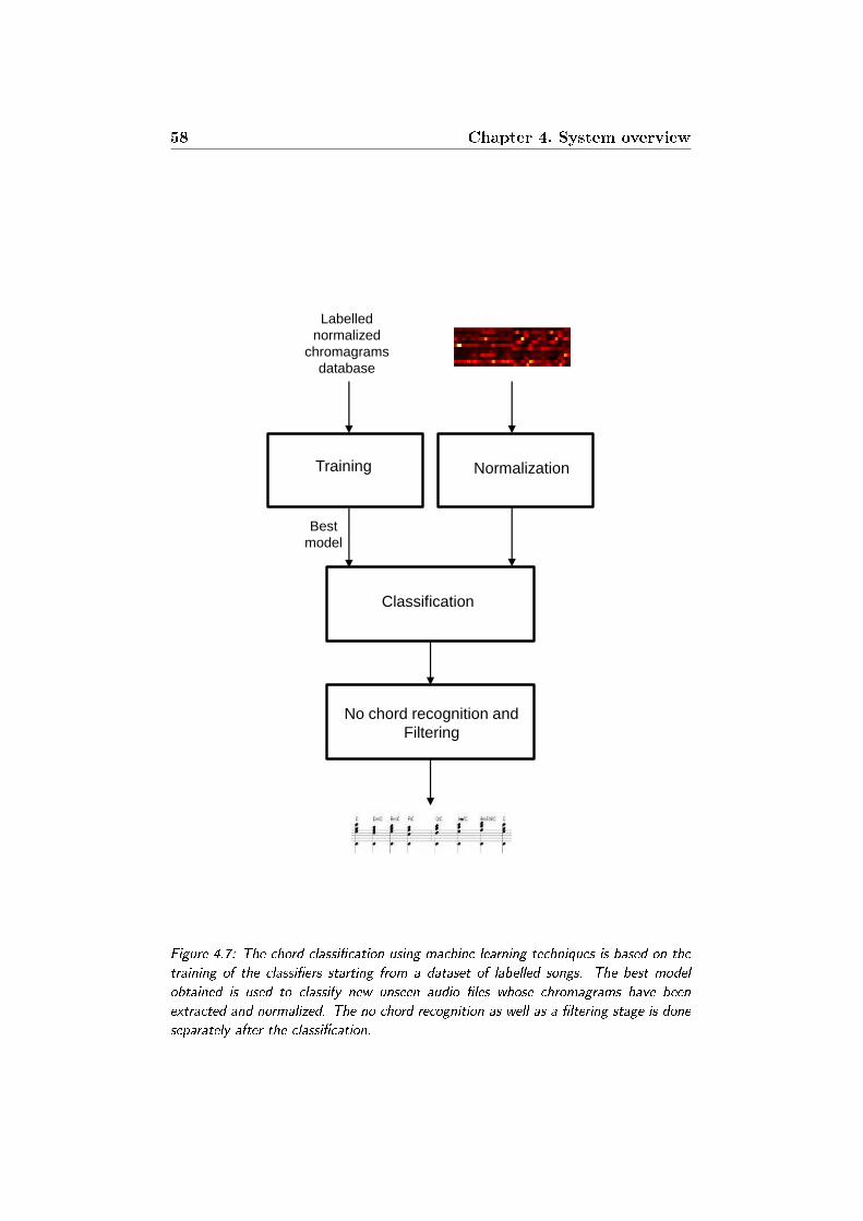
58 Chapter 4. System overview
Normalization
No chord recognition and
Filtering
Training
Labelled
normalized
chromagrams
database
Classification
Best
model
Figure 4.7: The chord classication using machine learning techniques is based on the
training of the classiers starting from a dataset of labelled songs. The best model
obtained is used to classify new unseen audio les whose chromagrams have been
extracted and normalized. The no chord recognition as well as a ltering stage is done
separately after the classication.
4.2. Machine learning classication 59
if they are Gaussian the input distribution needs to have zero mean and unit
variance. Feature normalization, thus, is an important pre-processing step
that can inuence the nal result of the classication algorithm.
The normalization of the features can be done in several ways. In order
to nd the normalization that best performs in our specic case, we tested
dierent strategies that will be addressed in the following subsections.
L-∞ normalization
The rst strategy that we tested is the normalization of the input features
dividing each element by the L-∞ norm of the corresponding feature vector.
Given the full chroma vector dataset that will be used in the training
stage D = (C136, C
236, ..., C
S36)′, where Cs is the 36-bins chromagram of a
generic song s and S is the number of songs, a feature vector is the vector
db that corresponds the the b-th column of the dataset D.
At the end of this normalization process, each feature vector will lie in the
[0,1] range. In particular, the feature vector db is normalized in the following
way:
dbnorm(i) =db(i)
maxdb(4.8)
for each i = 1, ..., N and b = 1, ..., 36.
Rescaling
Another option that we used for the normalization of the input features is to
force the values of each feature to be in the range [-1, 1]. This can be done
in two ways.
The rst way is to subtract the mean of each feature vector and then
divide it by the maximum value. In particular, given the feature vector dbthe normalization is done in two steps:
db(i) = db(i)−mean(db) (4.9)
and then:
db(i) =db(i)
max(db)(4.10)
for each i = 1, ..., N and b = 1, ..., 36.
The other way to perform this kind of normalization is the following.
Given
dbmax = max(db)
dbmin = min(db)
60 Chapter 4. System overview
the normalized feature vector can be obtained as:
dbscale(i) =2(dbmax − dbmin)
db(i)− dmin− 1 (4.11)
for each i = 1, ..., N and b = 1, ..., 36.
Binarization of the distribution
As described in chapter 3, the Deep Belief Network can take advantage
from an unsupervised pre-training strategy that has the goal of performing
a better initialization of the parameters.
The common Restricted Boltzmann Machine denition implies that the
input distribution has to be Binomial [5]. We decided, thus, to apply a
threshold on the values of the chroma vectors with the goal of forcing the
input distribution to be binary. In this way the greedy layer-wise pre-training
of a Deep Belief Network can be done. However, some information is lost in
the process, since the input distribution is not perfectly binary.
Given the generic chroma vector ci that corresponds to a row of the dataset
D, the new observations can be found as following:
cibin(b) =
1 ci(b) ≥ mean(ci)
0 otherwise
(4.12)
for each i = 1, ..., N , where N is the number of frames and b = 1, ..., 36.
Feature Standardization
A way that can be used to overcome the problem of the binarization of
the input distribution, is to substitute the Restricted Boltzmann Machine
at the input layer, with a Gaussian-Bernoulli RBM (GBRBM). However,
each input observation in this case, should be normalized to have zero mean
and unit variance since the estimation of the variance of the input noise
using Constrastive Divergence (CD1) is a dicult operation [20]. With this
normalization, the variance of the noise in the Energy expression of the
GBRBM becomes one and in this way the sampling of a visible observation
given the hidden units activations can be done just using the pre-sigmoid
activation. This kind of normalization is called feature standardization.
The feature standardization is usually done in two steps. First the mean
is subtracted from each element of the vector:
ci(b) = ci(b)−mean(ci) (4.13)
4.2. Machine learning classication 61
then each element is divided by the standard deviation of the vector:
cist(b) =ci(b)
std(ci)(4.14)
for each i = 1, ..., N and b = 1, ..., 36, where std(x) is the standard deviation
of the vector x.
4.2.2 Training and Evaluation Set creation
Machine learning classication algorithms need a training set of observations
in order to iteratively adjust the parameters of the model and an evaluation
set that is used to verify the generalization of the learnt model. The methods
that we used follow a supervised learning process. This means that it is
necessary to create two sets of chroma vectors and two sets of chords labels,
that indicates the corresponding class of each vector, that will be used for
the training phase.
In our specic case, the training and evaluation sets are generated starting
from a database of chromagrams extracted from previously labeled songs. In
particular, after each chromagram has been normalized as described in the
previous section, the training set is generated choosing random songs from
the labeled datasets taking the 36 bins chromagrams and the corresponding
chord labels. The no-chord chroma vectors and the corresponding labels are,
then, deleted from the resulting dataset.
The elements of the overall dataset are then randomly ordered, together
with the corresponding labels. This is done to avoid that the results of the
Stochastic Gradient Descent minimization algorithm are biased towards a
specic class. Starting from the obtained dataset, we split the elements to
create an actual training dataset, that will be used to adjust the parameters
of the network, and an evaluation dataset, that will be used to test the
generalization of the learnt model.
To summarize, at the end of the sets creation thus the results are:
• a matrix of dimensions Ntr x 36, where Ntr is the number of elements
in the training set and 36 is the number of features. Each chroma
vector is given as a row;
• a vector of length Ntr containing the correct labels of each observation
in the training matrix;
• a matrix of dimensions Nev x 36 where Nev is the number of elements
in the evaluation set;

62 Chapter 4. System overview
• a vector of length Nts containing the correct labels of each observation
in the test matrix.
They are given as input to the classiers that use them to compute the
training process that is described section 4.2.3.
Extended Training Dataset
The creation of a training set taking elements from random songs has the
drawback that the chroma vectors distribution is polarized towards certain
chords, as shown in Figure 5.10. In order to increase the number of ob-
servations for all possible chords, we also tried a strategy used by Bello in
[22].
The main idea behind the extension of the training set is to shift a chroma
vector to all possible positions. In this way, for each chord observation other
11 chroma vectors will be created from the original one. For example, for
the chroma vector that refers to the C major chord, we created other 11
chroma vectors corresponding to the remaining major chords shifting the
positions of the elements of the vector. In this way the numbers of major
chords observations is equalized, as well as the number of minor chords. Since
every major chord generates other major chords and minor chords generate
minor chords, the nal equalized number of major and minor elements will
not be equal, unless the overall number of major and minor chords is the
same before the extension. What is important, however, is that the number
of observations for every major chords is strongly increased (gure 5.13)
allowing the classiers to have a grater number of cases addressed in the
training stage that, theoretically, allows to have a gain in the performances.
The drawback of this method is that the dimension of the training set is
increased by a factor of 12 and the training process of the machine learning
algorithms will consequently take much more time.
4.2.3 Training and classication
The training and evaluation sets created in the previous phase are used by
the machine learning algorithms to learn the function that links each chroma
vector to the corresponding chord. The parameters are adjusted considering
only the training set, the evaluation set is used just an indicator of the
generalization of the model that is tested on unseen chroma vectors in order
to monitor the occurrence of overtting. The best model will be chosen as
the one that gives the lower classication error on the evaluation set. The
process is shown in Figure 4.8

4.2. Machine learning classication 63
The training process is done using Stochastic Gradient Descent minimiza-
tion algorithm proceeding byminibatches. This means that the input dataset
is scanned, and the parameters of the model are updated, considering each
time a limited number of input observations. This is usually done when
dealing with big datasets in order to allow matrix-matrix multiplies to be
used [20]. For each minibatch of data, the gradient of the cost function with
respect to the parameters of the model is computed and the parameters are
then updated in according to the Stochastic Gradient Descent update rule
(that we described in Chapter 3 in the equation 3.31). After all the mini-
batches has been considered, an epoch of the training process is completed.
At the end of every training epoch, the resulting model is tested on the eval-
uation set, computing the classication of each element as shown in gure
4.8. As we mentioned before, the resulting classication error is used as indi-
cator of the occurrence of overtting. In this case, in fact, the classication
error on the evaluation set instead of decreasing starts to grow indicating a
reduction of the generalization of the model. The best model is chosen to
be the one that gave the lower error on the evaluation set after a specied
number of epochs of the training process.
Once the classier has been trained in a supervised manner, the best
model is saved and it is used to compute the chord identication of new
unseen songs.
The output units of each machine learning method are associated to each
chord class. With this interpretation, the classication is obtained calculat-
ing the posterior probabilities of each chord class, given the chroma vector
as observation, using the parameters of the best model θ obtained after the
training phase. The chord class that has the maximum probability is chosen
as classication. In particular, for the r-th chroma vector cr:
lr = argmaxhP (Chord = h|Chroma = cr; θ) (4.15)
where h corresponds to the chord label, that is an integer number that ranges
from 0 to 23 indicating the rst 12 numbers the major chords and the suc-
cessive 12 the minor chords. In the case of Logistic Regression, the posterior
probability is computed straight-forward by means of the softmax function
as described in section 3.3.1 in the equation 3.27. In the case of One-Hidden
Layer Multilayer Perceptron and Deep Belief Network the posterior proba-
bility is also computed as a softmax function, since the Logistic Regressor
is used as output layer of the networks, but this time having as input the ac-
tivations of the hidden units of the last hidden layer. In both cases, they are
obtained by means of a forward pass of the network, computing recursively
the activations of each hidden units of every hidden layer, starting from the
64 Chapter 4. System overview
chroma vector observation. In particular, for the One-Hidden Layer Multi-
layer Perceptron the classication is obtained as:
lr = argmaxh(softmaxh(b(2) + W (2)(tanhh(b(1) + W (1)x)))) (4.16)
where W (1), b(1) indicates the parameters of the best model for the rst layer
and W (2), b(2) indicates the parameters of the best model for the second layer.
For the Deep Belief Network the expression is similar with the dierence that
instead of tanh the hidden units activation function is the sigm and that the
recursion on x is applied for every hidden layer in the network. This time
the number of layers will be arbitrary.
The result of the classication for each chroma vector, is stored in a vector
of labels lc each one corresponding to the label of the classied chord. Since
the classiers are able to recognize just the chords elements, this vector is
then modied at the following stage in order to add the detected no-chord
labels and to address temporal correlation by means of a ltering stage.
The machine learning algorithms have been implemented in Python using
the Theano library [6]. Theano is a powerful tool that can be used to com-
pute mathematical expressions in an easy way. It works starting from the
allocation of symbolic variables that point to Python objects and operations
that are connected to create a computational graph that represents generic
functions. Thanks to this structure, Theano is able to compute automatic
dierentiations of mathematical functions and to perform optimizations for
numerical stability as well as creating compiled C code that allows to have
better performances. More details can be found in [6].
Each of the three machine learning algorithms that we tested are python
classes that are initialized in the method that computes the learning pro-
cess. The training and test sets as well as the vector labels computed in
the previous phase are loaded in Theano shared variables. They are a par-
ticular type of Theano variables that can be used to create computational
graphs but they also have an internal value that can be accessed by dierent
functions. The loading of the datasets in shared variables allows to create
computational graphs dening Theano functions that are used to perform
the training and testing phases. In the following subsections we will give
some details about each classier.
Logistic Regression
Logistic Regression is the simplest of the three models. It is used as output
layer for the One Hidden Layer Multilayer Perceptron as well as the Deep
Belief Networks.
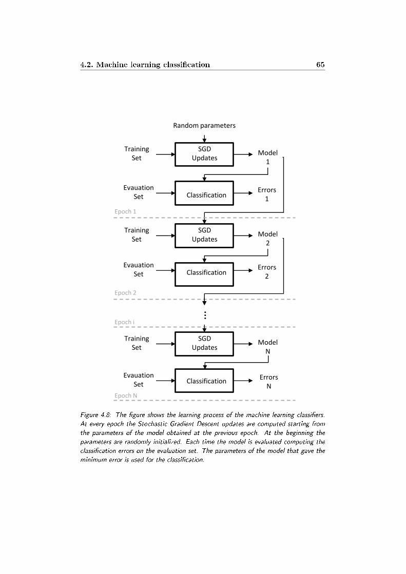
4.2. Machine learning classication 65
SGD Updates
Training Set
Model N
Evauation Set Classification
Errors N
…
Random parameters
SGD Updates
Training Set
Model 1
Evauation Set Classification
Errors 1
SGD Updates
Training Set
Model 2
Evauation Set Classification
Errors 2
Epoch 1
Epoch 2
Epoch N
Epoch i
Figure 4.8: The gure shows the learning process of the machine learning classiers.
At every epoch the Stochastic Gradient Descent updates are computed starting from
the parameters of the model obtained at the previous epoch. At the beginning the
parameters are randomly initialized. Each time the model is evaluated computing the
classication errors on the evaluation set. The parameters of the model that gave the
minimum error is used for the classication.

66 Chapter 4. System overview
After the datasets has been loaded in Theano shared variables, the train-
ing phase starts with the instantiation of the Logistic Regression class. In
particular:
• the weights W are initialized as a matrix of zeros of dimensions 36 x
24, where 36 is the dimension of each chroma vector and 24 the number
of chord classes;
• the biases b are initialized as a vector of zeros of length 24;
• the posterior probabilities of each chord class is dened as a symbolic
Theano expression that denes the softmax function of crW + b;
• the predicted class is dened as a symbolic Theano expression that
denes the argmax of the posterior probabilities.
• the cost function is also a symbolic Theano expression that denes the
negative log likelihood (chapter 3). The only dierence with respect to
the denition is that the mean is used instead of the sum in order to
improve the performances of the minimization algorithm, as suggested
in [20].
The parameters of the model W and b are loaded in Theano shared vari-
ables. In this way, they can be used to create a Theano computational graph
for the denition of symbolic expressions needed in the optimization. At the
same time, their values can be updated at every iteration of the training
phase.
The main advantage of using Theano for this kind of applications is that,
thanks to the creation of a computational graph, the gradient of the cost
function with respect to the parameters is automatically computed starting
from the denition of the symbolic expression.
The gradients are used to compute the update expressions of the param-
eters. Once the updates symbolic expressions has been dened, a Theano
function that computes the training of a minibatch is dened simply by giv-
ing as input the index of a minibatch, the update symbolic expression and the
symbolic variables representing the input observations and labels belonging
to a minibatch. The function returns the number of errors considering the
training minibatch. At the same way is dened a test function as a Theano
function with the only dierence that this time no update of the parameters
is done.
The train function is then called for each minibatch index for a predened
number of epochs. Each time the testing function is also called, visualizing
the number of errors done by the learnt model.
4.2. Machine learning classication 67
Summarizing, the parameters that needs to be dened for the training
and testing of a Logistic Regression are:
• the training and test sets of chroma vectors observations and labels
loaded in Theano shared variables;
• the learning rate used by SGD dened as a real number;
• the size of a minibatch dened as an integer number;
• the number of epochs of the training process dened as an integer
number.
One-Hidden Layer Multilayer Perceptron
The One Hidden Layer Multilayer Perceptron is constructed dening a Hid-
den Layer class that will be used as hidden layer and instantiating the Logis-
tic Regression Class that we saw in the previous subsection to be the output
layer.
The attributes of the Hidden Layer class are:
• a matrix of weights Whid of dimensions 36 x Nhid, where Nhid is the
number of hidden units. This time, parameters are not set to zero
but they are initialized in a dierent way depending on the activation
function chosen [14]. In our case, since the activation function is a
tanh the parameters are initialized as random number in the interval[−√
6Nvisible+Nhidden
,√
6Nvisible+Nhidden
];
• a vector of biases bhid that has a length equal to the number of hidden
units;
• a symbolic variable that computes the activations of the hidden units
as dened in chapter 3.
Like in the Logistic Regression case, the parametersWhid and bhid are loaded
in Theano shared variables.
The One Hidden Layer Multilayer Perceptron class is composed by:
• a hidden layer that is an instance of the Hidden Layer class;
• an output layer that is an instance of the Logistic Regression class;
• the symbolic expression of the L2-norm of the parameters used for
weight decay (see chapter 3);
68 Chapter 4. System overview
• the expressions for the negative log likelihood and the errors that are
the same of the Logistic Regression class.
The One Hidden Layer Multilayer Perceptron is trained by minibatch
dening the Theano functions in the same way of the logistic regression
case. The dierence in this case is that the cost function takes into account
the regularization term of weight decay as dened in chapter 3. The updates
are dened as a list of elements for each parameter respectively of the hidden
and output layer.
Summarizing, the parameters that needs to be dened for the training
and testing of a One Hidden Layer Multilayer Perceptron are:
• the training and test sets of chroma vectors observations and labels
dened as Theano shared variables;
• the learning rate used by SGD dened as a real number;
• the size of a minibatch dened as an integer number:
• the number of epochs of the training process dened as an integer
number;
• the number of hidden units of the hidden layer dened as an integer
number;
• the regularization coecient used for weight decay dened as real num-
ber.
Deep Belief Network
The creation of the Deep Belief Network is based on the Logistic Regres-
sion, Hidden Layer and Restricted Boltzmann Machine classes. The Logistic
Regression and Hidden Layer classes are the ones previously described.
The attributes of the Restricted Boltzmann Machine class are:
• a weight matrix WRBM with dimensions depending on the number of
visible and hidden units. The weights are initialized to be random num-
bers belonging to the interval[−4√
6Nvisible+Nhidden
, 4√
6Nvisible+Nhidden
].
This initialization has been proven to be a good choice in case of sig-
moid activation functions [14];
• a hidden bias vector bhid and a visible bias vector bvis both initialized
as vectors of zeros;
• the number of hidden and visible units.
4.2. Machine learning classication 69
The Deep Belief Network class is constructed dening the following ele-
ments:
• a list of Hidden Layer classes that share the parameters with the Deep
Belief Network is created;
• a list of Restricted Boltzmann Machine classes. These classes do not
share the visible bias vector with the Deep Belief Network;
• a Logistic Regression class is dened as output layer.
The parameters of all the classes used are loaded in Theano shared variables.
The unsupervised pre-training phase is done using Contrastive Divergence-
1 as described in chapter 3. The Restricted Boltzmann Machine class pro-
vides functions that computes each step of the algorithm. In particular, the
functions compute:
• the Free Energy of the model given the visible sample;
• the up-propagation (positive phase) and down-propagation(negative
phase) that return the mean activations of visible and hidden units;
• the sampling of visible and hidden units given by means of the mean
activations.
For each layer of the network Restricted Boltzmann Machines are trained
in an unsupervised manner dening Theano functions that update the pa-
rameters of the Network.
The supervised training of a Deep Belief Network is done in the same way
of the One Hidden Layer Multilayer Perceptron.
The Deep Belief Network with Gaussian input units is dened in same
way as before with the only dierence that the rst element in the Restricted
Boltzmann Machines list is a Gaussian-Bernoulli Restricted Boltzmann Ma-
chine. The dierences between the two classes regard the implementation of
the functions used to compute each step of the CD-1 algorithm. In particu-
lar, the free energy computation and the sampling of the visible units given
the hidden are modied as described in chapter 3.
Summarizing, the parameters that needs to be dened for the training
and testing of a Deep Belief Network are:
• the training and test sets of chroma vectors observations and labels;
• the learning rate used by SGD dened as a real number;
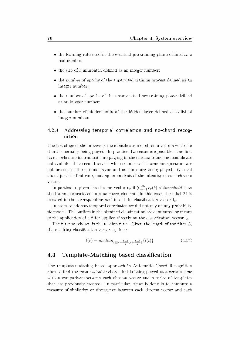
70 Chapter 4. System overview
• the learning rate used in the eventual pre-training phase dened as a
real number;
• the size of a minibatch dened as an integer number;
• the number of epochs of the supervised training process dened as an
integer number;
• the number of epochs of the unsupervised pre-training phase dened
as an integer number;
• the number of hidden units of the hidden layer dened as a list of
integer numbers.
4.2.4 Addressing temporal correlation and no-chord recog-
nition
The last stage of the process is the identication of chroma vectors where no
chord is actually being played. In practice, two cases are possible. The rst
case is when no instruments are playing in the chroma frame and sounds are
not audible. The second case is when sounds with harmonic spectrum are
not present in the chroma frame and no notes are being played. We deal
about just the rst case, making an analysis of the intensity of each chroma
vector.
In particular, given the chroma vector cr if∑36
b=1 cr(b) < threshold then
the frame is associated to a no-chord element. In this case, the label 24 is
inserted in the corresponding position of the classication vector lc.
In order to address temporal correlation we did not rely on any probabilis-
tic model. The outliers in the obtained classication are eliminated by means
of the application of a lter applied directly on the classication vector lc.
The lter we chosen is the median lter. Given the length of the lter L,
the resulting classication vector is, then:
l(r) = mediant∈[r−L−12,r+L−1
2] l(t) (4.17)
4.3 Template-Matching based classication
The template-matching based approach in Automatic Chord Recognition
aims to nd the most probable chord that is being played at a certain time
with a comparison between each chroma vector and a series of templates
that are previously created. In particular, what is done is to compute a
measure of similarity or divergence between each chroma vector and each

4.3. Template-Matching based classication 71
chord template. This kind of approach has been introduced in the rst
chord recognition system by Fujishima in [10]. In our work we modied
the template matching classication process used by Oudre, Grenier and
Fevotte in [32] applying a temporal domain lter directly to the resulting
classication vector instead of applying it to the matrix of distances, as done
by Harte in [17], and we used not normalized template models.
This method has some advantages as well as disadvantages. In particular,
the advantage is that they are exible methods since they do not depend
on a the creation of a training set but, on the other hand, the correctness
of the classication is strongly dependent from the choice of the template
model and the distance measure chosen. Moreover, the presence of noise in
the chroma vectors inuences the quality of the nal classication.
In the following subsection we will briey describe the phases regarding
the classication process.
Template models
The rst step in the template based classication is the creation of a model of
the ideal chroma vectors. The simplest model that can be created is a binary
model that is based on the denition of chord. We know that with chord is
meant the simultaneus execution of at least three notes at the certain time.
The template binary model for a chroma vector representing a particular
chord h is, thus, a 12-dimensional vector dened as:
th[m] =
1 if the m-th note belongs to the chord k
0 otherwise
(4.18)
An example of chord template for is shown in gure 4.9.
Measure of distance
Once the template models have been created, the following step is to compute
a measure of distance. In the literature several measures have been proposed,
we chosen the Kullback-Leibler (KL) divergence since it has been proven to
be the best performing one [32].
The KL divergence is a similarity measure that gives an indication of the
dierence between two probability distributions. The KL divergence is not
symmetric. In particular, given two vectors x and y the generalized KL
divergence is dened as:
KL(x|y) =∑m
(x(m) log
(x(m)
y(m)
)− x(m) + y(m)). (4.19)
Figure 4.9: The gure shows the binary template model for the C major chord, where
the pitch classes corresponding to the notes belonging to the chord have value 1, the
remaining have value 0
If x and y are two probability distributions KL(x|y) is a measure of infor-
mation lost when y is used to approximate x.
In our case, the KL divergence is computed between the 24 chord tem-
plates and each chroma vector. In particular the distance matrix M is ob-
tained such that
M(h, r) = KL(th|cr) (4.20)
for each chord h = 0, ..., 24 and each frame r = 1, ..., R where R is the
number of chroma frames.
The classication is performed analyzing the distance matrix. In particu-
lar, for each frame, the chord corresponding to the template vector that gave
the minimum value is chosen: lc(r) = argminh(M(h, r))
No-chord recognition and temporal correlation
The last step in the classication process consists in the identication of the
no chords elements. Even in this case we did not rely on any template model
of the no-chord chroma vector. We analyzed, like in the machine learning
case the sum each chroma vector and, in particular if∑
b cr(b) < threshold
then the result of the classication will be a no-chord element.
Once the classication vector is computed, a nal ltering step is done in
order to eliminate chords outliers on the resulting classication. This is done
in the same way of the machine learning approach by means of the equation
4.17.
Chapter 5
Experimental results
This chapter is dedicated to the description of the experiments that we per-
formed as well as the denition of the evaluation metrics and the specic
experimental setup we used.
The chapter is divided in four sections. In the rst section we will present
the evaluation metrics used to measure the performances of the approaches
that we tested. They are the Weighted Average Overlap Ratio (WAOR) and
the Segmentation Quality (SQ) and will be described in section 5.1.
The other sections are dedicated to the description of the experiments
done and to the expositions of the results. Section 5.2 and 5.3 describe the
experimental setup used in the feature extraction, normalization and feature
selection. The second section (section 5.2) regards the feature extraction
phase. The third section (section 5.3) is about the normalization and feature
selection. The last section (section 5.4) is dedicated to the experiment to
evaluate the performances and the robustness of the approach.
5.1 Evaluation metrics
In order to compute an evaluation of the chords transcription, two metrics
have been used. The rst evaluation measure, the WAOR score, is based on
a metric called Relative Correct Overlap (RCO). This evaluation is computed
against a ground truth annotation. The chord transcription process produces
a segmentation of the song where each segment is associated to a detected
chord. The goal of RCO is to produce a value that is an indication of how
long correctly classied segments of chords remain overlapped to the ones of
the ground truth annotation. The measure is normalized with respect to the
song duration. A good chord transcription of a song, therefore, will result in
a high value of the RCO score: if the transcription is perfectly overlapped
73
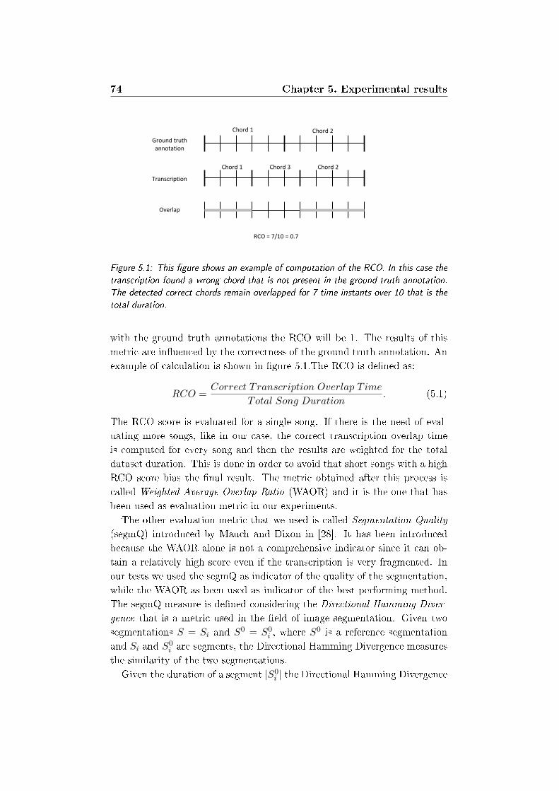
74 Chapter 5. Experimental results
Chord 1 Chord 2
Chord 1 Chord 3 Chord 2
Ground truth annotation
Transcription
Overlap
RCO = 7/10 = 0.7
Figure 5.1: This gure shows an example of computation of the RCO. In this case the
transcription found a wrong chord that is not present in the ground truth annotation.
The detected correct chords remain overlapped for 7 time instants over 10 that is the
total duration.
with the ground truth annotations the RCO will be 1. The results of this
metric are inuenced by the correctness of the ground truth annotation. An
example of calculation is shown in gure 5.1.The RCO is dened as:
RCO =Correct Transcription Overlap T ime
Total Song Duration. (5.1)
The RCO score is evaluated for a single song. If there is the need of eval-
uating more songs, like in our case, the correct transcription overlap time
is computed for every song and then the results are weighted for the total
dataset duration. This is done in order to avoid that short songs with a high
RCO score bias the nal result. The metric obtained after this process is
called Weighted Average Overlap Ratio (WAOR) and it is the one that has
been used as evaluation metric in our experiments.
The other evaluation metric that we used is called Segmentation Quality
(segmQ) introduced by Mauch and Dixon in [28]. It has been introduced
because the WAOR alone is not a comprehensive indicator since it can ob-
tain a relatively high score even if the transcription is very fragmented. In
our tests we used the segmQ as indicator of the quality of the segmentation,
while the WAOR as been used as indicator of the best performing method.
The segmQ measure is dened considering the Directional Hamming Diver-
gence that is a metric used in the eld of image segmentation. Given two
segmentations S = Si and S0 = S0
i , where S0 is a reference segmentation
and Si and S0i are segments, the Directional Hamming Divergence measures
the similarity of the two segmentations.
Given the duration of a segment |S0i | the Directional Hamming Divergence

5.2. Feature extraction experiments 75
is dened as:
h(S||S0) =
NS∑i=1
(|S0i | −max
j|S0i ∩ Sj |). (5.2)
Starting from the Directional Hamming Divergence, the segmQ measure for
the chord recognition task is dened as:
SQ(S||S0) = 1− 1
Tmaxh(S||S0), h(S0||S) ∈ [0, 1] (5.3)
5.2 Feature extraction experiments
The rst experiments that we performed focus on the feature extraction
phase. We evaluated the performances of the dierent ways to extract the
chromagram that we described in Chapter 4 using, as classication method,
the template matching based approach also described in Section 4.3. The
chromagram computational baseline that best performed in these tests has
been adopted for the experiments regarding the classication phase described
in section 5.3.
5.2.1 Dataset
For the evaluation of the system we used songs taken from two manually
annotated datasets available on line. The rst dataset is the annotated
Beatles discography that has been used in the past few years for the MIREX
competition about chord recognition. The other dataset is composed by 5
Robbie Williams albums, the transcriptions of the rst two albums has been
provided by Davies in [9] it has been successively extended by Di Giorgi in [2].
The tests have been done on a bench of 74 songs extracted by both datasets,
following the strategy used also in the successive tests about machine learning
approaches where a training set is needed.
5.2.2 Experimental setup
The choice of the parameters for the chromagrams extraction has been done
in the following way. As we described in Section 3.2.3, the notes between C0
and C7 have values in the range between 30Hz and 2000Hz. Thus the signal
has been downsampled to 11025Hz without having loss of information. The
STFT algorithm can be implemented eciently using the FFT computation
if the window length is a power of 2 (Section 3.2.1). The closer value in our
case is 212 = 4096, so the window length for the STFT computation has
been chosen to be Lw = 4096. The hopsize Hop is chosen to be Hop = 512
that, considering our downsampling frequency, is ∼ 0, 05sec.
76 Chapter 5. Experimental results
Regarding the constant-Q transform parameters, the minimum frequency
has been chosen to be f0 = 73.42Hz that corresponds to the note D2. The
constant-Q transform spans three octaves starting from the minimum fre-
quency, that corresponds to having 108 frequency bins in the resulting matrix
Xcq(k, r) with a resolution of 36 bins per octave.
Considering the HPSS algorithm, the choice of the parameters has been
the same used in [29], in particular γ = 0.3 and α = 0.3. Regarding the
choice of the number of iterations of the algorithm Nhpss, we rst tried to
nd a relation between its value and the mean harmonicity of the songs.
However we did not nd any relation between the two parameters, as shown
in Figure 5.2. The value, thus, has been empirically chosen to be 25.
The last choices regards the A-weighing parameters. As described in Sec-
tion 4.1.2, the only parameter that needs to be chosen is the reference power,
that we decided to choose to be the standard value of Rp = 10−12.
The choice of the lter lengths has also been empirically chosen. In partic-
ular, the averaging and median lters showed to have the best performances
for a length of 30 samples. The geometric mean for a lower length of 15.
Finally, the harmonic mean of 5 samples.
The last choices for the parameters regards the classication methods. In
particular the only parameters that have to be chosen are the threshold for
the no-chord recognition and the length of the median lter applied to the
classication vector to address temporal correlation. Both the parameters
have been empirically chosen. In particular, the threshold has been set to
thresh = 10−2. The length of the lter has been selected to be of 31 samples.
5.2.3 Results
We performed a preliminary experiment that we conducted concerns the per-
formance of the three types of chromagrams described in Section 4.1 without
any ltering stage applied. The rst method considers the chromagram com-
puted using the standard baseline, referenced in Table 5.1 as Chroma. The
second method computes the chromagram starting from the harmonic com-
ponents extracted by means of the HPSS and is referenced in Table 5.1 as
Chroma + HPSS. The last method makes use of the A-weighting of the log
spectrum and is referenced in the Table 5.1 as A-Weighted Chroma.
To evaluate the performances we tested the three methods using the
straight forward template-matching method described in Section 4.3. We
evaluated the Weighted Average Overalp Ratio and the Segmentation Qual-
ity, denoted respectively as (WAOR) and (segmQ). The expected results are
poor performances, due to the lack of a denoising stage. The results are

5.2. Feature extraction experiments 77
Figure 5.2: In this plot each point represent a song where the mean harmonicity and
the best number of iterations of the HPSS algorithm are shown. A correlation between
these two variables is not evident. The most of the songs have best performances when
25 iterations are done.
showed in Table 5.1.
WAOR segmQ
Chroma 0.512 0.619
Chroma + HPSS 0.522 0.636
A-Weighted Chroma 0.500 0.645
Table 5.1: The table shows the performances obtained by the chromagrams without
any applied lter.
The performances are very poor, since it is a frame-wise classication
without the use of any ltering stage. The chromagram computed start-
ing from the harmonic signal obtained the best performance regarding the
WAOR while the A-Weighted chroma obtained the best Segmentation Qual-
ity score.
In order to evaluate the eect of the application of temporal domain lters,
the second experiment has been to add a ltering stage to the chromagram
computation. First, we performed this stage to the 36 bins chromagram
before the reduction to 12 pitch classes. For each of the previously tested
chromagrams, we tried the four lters types we described in Section 4.1.3.

78 Chapter 5. Experimental results
Thanks to the application of a ltering stage, we expect to have a gain in the
performances relative to the previous test. The results are shown in Table
5.2.
WAOR segmQ
Chroma Avg 0.612 0.718
Chroma Med 0.650 0.733
Chroma Geom 0.640 0.725
Chroma Harm Mean 0.600 0.684
Chroma + HPSS Avg 0.613 0.711
Chroma + HPSS Med 0.649 0.735
Chroma + HPSS Geom 0.633 0.722
Chroma + HPSS Harm Mean 0.591 0.682
A-Weighted Chroma Avg 0.580 0.721
A-Weighted Chroma Med 0.591 0.740
A-Weighted Chroma Geom 0.590 0.740
A-Weighted Chroma Harm Mean 0.556 0.708
Table 5.2: The table shows the performances obtained by the chromagrams with a
ltering phase computed on the 36 bins representation before the folding to 12 pitch
classes. The averaging lter is denoted as Avg, the median lter as Med, the geometric
mean lter as Geom and the harmonic mean as Harm Mean.
The ltering stage allowed to have a gain in the performance, as expected.
The median lter has been the best performing one, followed by the geomet-
ric mean that performed better than the averaging lter and the harmonic
mean that had the poorest performance. The ltering stage allowed to ll the
performance gap between the chromagrams of the previous experiment since
the best WAOR score has been obtained by the standard chromagram when
applied median lter. The result however is very close to the one obtained
by the chromagram computed on the extracted harmonic components. The
best segmQ score, instead, is obtained by the A-weighted chromagram when
using median lter or geometric mean.
In the last experiment we performed the ltering stage after the folding
to 12 pitch classes of the chromagram, in order to see if the results change
with respect to the performances obtained by the ltering done before the
folding. The results are shown in Table 5.3.
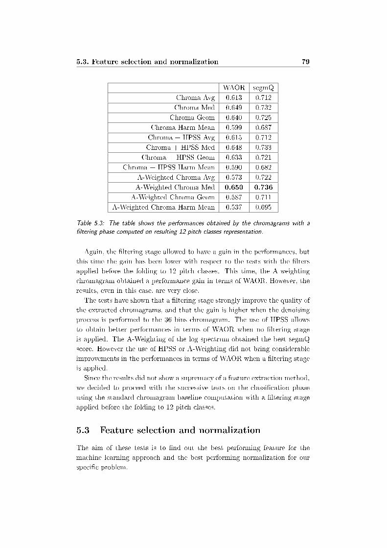
5.3. Feature selection and normalization 79
WAOR segmQ
Chroma Avg 0.613 0.712
Chroma Med 0.649 0.732
Chroma Geom 0.640 0.725
Chroma Harm Mean 0.599 0.687
Chroma + HPSS Avg 0.615 0.712
Chroma + HPSS Med 0.648 0.733
Chroma + HPSS Geom 0.633 0.721
Chroma + HPSS Harm Mean 0.590 0.682
A-Weighted Chroma Avg 0.573 0.722
A-Weighted Chroma Med 0.650 0.736
A-Weighted Chroma Geom 0.587 0.711
A-Weighted Chroma Harm Mean 0.537 0.695
Table 5.3: The table shows the performances obtained by the chromagrams with a
ltering phase computed on resulting 12 pitch classes representation.
Again, the ltering stage allowed to have a gain in the performances, but
this time the gain has been lower with respect to the tests with the lters
applied before the folding to 12 pitch classes. This time, the A-weighting
chromagram obtained a performance gain in terms of WAOR. However, the
results, even in this case, are very close.
The tests have shown that a ltering stage strongly improve the quality of
the extracted chromagrams, and that the gain is higher when the denoising
process is performed to the 36 bins chromagram. The use of HPSS allows
to obtain better performances in terms of WAOR when no ltering stage
is applied. The A-Weighting of the log spectrum obtained the best segmQ
score. However the use of HPSS or A-Weighting did not bring considerable
improvements in the performances in terms of WAOR when a ltering stage
is applied.
Since the results did not show a supremacy of a feature extraction method,
we decided to proceed with the successive tests on the classication phase
using the standard chromagram baseline computation with a ltering stage
applied before the folding to 12 pitch classes.
5.3 Feature selection and normalization
The aim of these tests is to nd out the best performing feature for the
machine learning approach and the best performing normalization for our
specic problem.
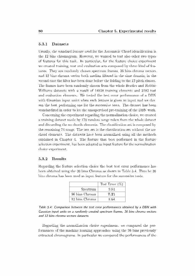
80 Chapter 5. Experimental results
5.3.1 Datasets
Usually, the standard feature used for the Automatic Chord identication is
the 12 bins chromagram. However, we wanted to test also other two types
of features for this task. In particular, for the feature choice experiment
we created training, test and evaluation sets composed by three kind of fea-
tures. They are randomly chosen spectrum frames, 36 bins chroma vectors
and 12 bins chroma vector both median ltered in the time domain, in the
second case the lter has been done before the folding to the 12 pitch classes.
The frames have been randomly chosen from the whole Beatles and Robbie
Williams datasets with a result of 14858 training elements and 3183 test
and evaluation elements. We tested the test error performance of a DBN
with Gaussian input units when each feature is given as input and we cho-
sen the best performing one for the successive tests. The dataset has been
standardized in order to let the unsupervised pre-training of the DBN work.
Concerning the experiment regarding the normalization choice, we created
a training dataset made by 170 random songs taken from the whole dataset
and discarding the no-chords elements. The classication set is composed by
the remaining 74 songs. The test set is the classication set without the no-
chord elements. The datasets have been normalized using all the methods
explained in Chapter 4. The feature that best performed in the feature
selection experiment, has been adopted as input feature for the normalization
choice experiment.
5.3.2 Results
Regarding the feature selection choice the best test error performance has
been obtained using the 36 bins Chroma as shown in Table 5.4. Thus he 36
bins chroma has been used as input feature for the successive tests.
Test Error (%)
Spectrum 9.84
36 bins Chroma 7.21
12 bins Chroma 8.64
Table 5.4: Comparison between the test error performances obtained by a DBN with
Gaussian input units on a randomly created spectrum frames, 36 bins chroma vectors
and 12 bins chroma vectors datasets.
Regarding the normalization choice experiment, we compared the per-
formances of the machine learning approaches using the 36 bins previously
extracted chromagrams. In particular we compared the performances of the

5.3. Feature selection and normalization 81
Logistic Regression (LR), Single Hidden Layer Multilayer Perceptron (MLP),
Deep Belief Network (DBN). For the reasons we described in section 4.2.1.
The pretraining of the DBN has been possible only for the binarized dataset
using binary visible units RBM and for the standardized one using Gaussian-
Bernoulli RBM, in the other cases no pretraining of the network has been
done.
In order to test the MLP and the DBN with the same number of hidden
units but without having a penalizing computational time, we chosen to
use a MLP with 150 hidden units and a DBN made by 3 hidden layers of
dimensions [50, 50, 50]. In this way also the DBN has 150 hidden units, but
they are distributed over the three layers.
The netuning learning rate has been chosen to be 0,01 for every method.
For every method we used the best performing model to evaluate the classi-
cation set.
In both cases we used WAOR and segmQ as the evaluation metrics. The
results are shown in table 5.5.
LR MLP DBN
L-∞ WAOR 0.669 0.696 0.719
L-∞ segmQ 0.741 0.749 0.760
FS1 WAOR 0.676 0.703 0.722
FS1 segmQ 0.756 0.766 0.769
FS2 WAOR 0.695 0.706 0.711
FS2 segmQ 0.751 0.752 0.760
STD WAOR 0.713 0.723 0.726(*)
STD segmQ 0.757 0.762 0.762(*)
BIN WAOR 0.698 0.702 0.701(**)
BIN segmQ 0.755 0.756 0.756(**)
Table 5.5: The table shows the comparison between the performances obtained with
the dierent normalization strategies by the machine learning approaches. Where no
star is present, the DBN did not have a pre-training stage. The (*) indicates that
the DBN has been pre-trained having Gaussian input units, the (**) indicates that has
been pre-trained having binary units. The L-∞ norm is described in Section 4.2.1,
FS1 and FS2 are the rst and second methods described in Section 4.2.1, STD is the
standardization (section 4.2.1), BIN the binarization (section 4.2.1).
The results show that the best normalization type for the problem in terms
of WAOR is the standardization while in terms of segmQ is the FS1. The
DBN has been the best performing method. However, with the standardiza-
tion the MLP also received a gain the performances almost equalizing the

82 Chapter 5. Experimental results
DBN one. In order to test the performances of the machine learning tech-
niques as well as the robustness of the approach we decided to proceed using
the feature standardization as normalization technique since it gave the best
WAOR score.
5.4 Performance comparison and robustness of the
approach
In this section we present the experiments we performed to compare the
performances of the machine learning methods with respect to the state of
the art template-matching approaches and to evaluate the robustness of our
approach.
The dependence on a training set could be the main drawback of using
machine learning techniques. In order to test how the performances of these
methods change with respect to the training set variation we performed two
dierent experiments. In the rst one, we created dierent random datasets,
in the second one we evaluated how the performances of the best performing
machine learning method change with respect to the cardinality variation of
the training set.
As last experiment, we evaluated how the performances of the best per-
forming method change when the training set is extended using the Extended
Training Dataset strategy described in Section 4.2.2.
5.4.1 Experiment 1: performance evaluation on various datasets
In this experiment we created dierent random datasets in order to evaluate
the robustness of the machine learning techniques, each time doing a com-
parison with template-matching based methods. In particular we created
other 5 mixed datasets with the same approach of the previous tests taking
every time 170 songs as training set and 74 songs as classication set from
the whole Beatles and Robbie Williams dataset.
The cardinality of the datasets is the following:
• dataset 1: training set size = 462169, evaluation set size = 198072;
• dataset 2: training set size = 447036, evaluation set size = 191586;
• dataset 3: training set size = 454654, evaluation set size = 194850;
• dataset 4: training set size = 456109, evaluation set size = 195474;
• dataset 5: training set size = 455620, evaluation set size = 195266;
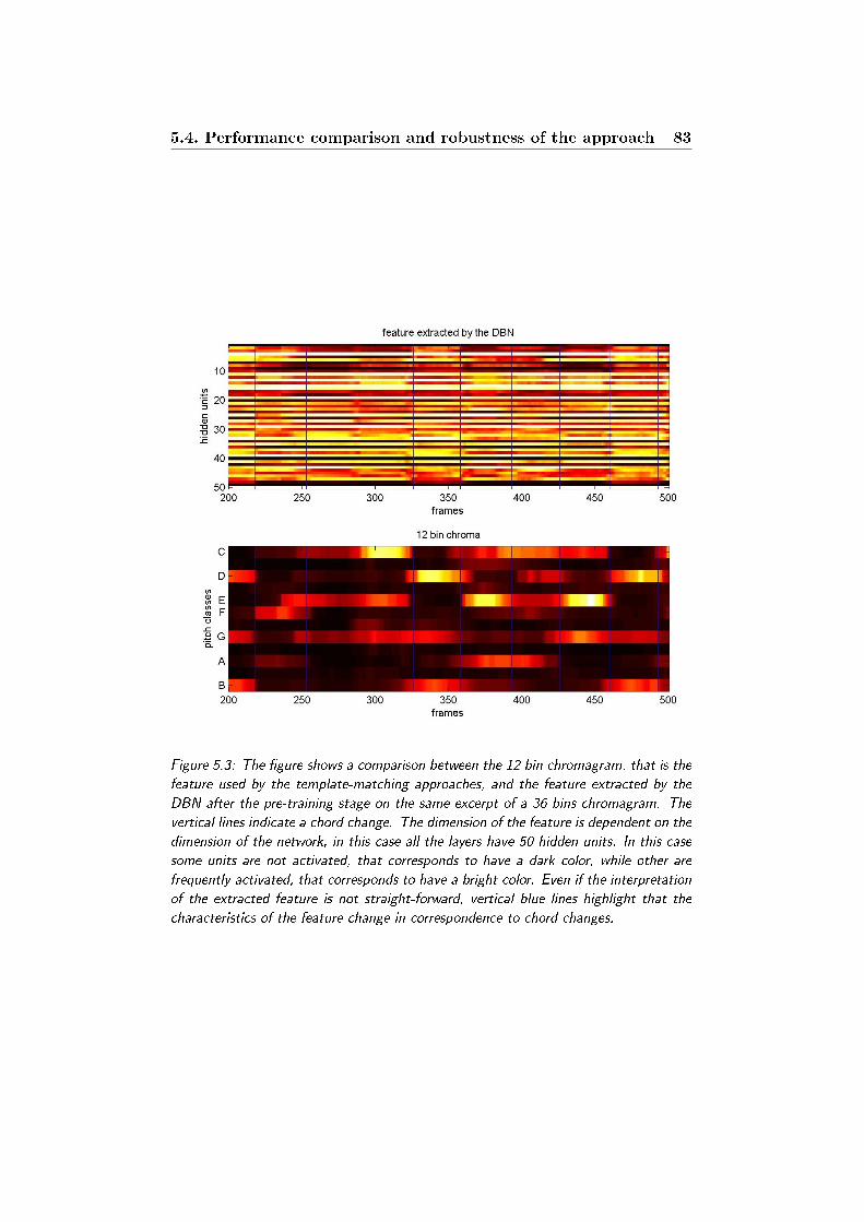
5.4. Performance comparison and robustness of the approach 83
Figure 5.3: The gure shows a comparison between the 12 bin chromagram, that is the
feature used by the template-matching approaches, and the feature extracted by the
DBN after the pre-training stage on the same excerpt of a 36 bins chromagram. The
vertical lines indicate a chord change. The dimension of the feature is dependent on the
dimension of the network, in this case all the layers have 50 hidden units. In this case
some units are not activated, that corresponds to have a dark color, while other are
frequently activated, that corresponds to have a bright color. Even if the interpretation
of the extracted feature is not straight-forward, vertical blue lines highlight that the
characteristics of the feature change in correspondence to chord changes.

84 Chapter 5. Experimental results
For each dataset we compared the performance of the machine learn-
ing techniques with the template matching based approaches on the same
dataset. In particular we used the methods proposed in [32] denoted as
(OT), in [33] denoted as (OP), and the one described in Chapter 4 (KL).
In order to show how the use of a temporal lter improve the classica-
tion we also evaluated the rst method (OT) without any ltering stage
(OTnf). All these methods are applied on the 12 bins chromagram normal-
ized between [0,1] as required by the chord template models formulation and
KL-divergence. The machine learning techniques, instead, use the 36-bins
standardized chromagram as input feature. In both cases the chromagrams
has been median ltered during the extraction. In gure 5.3 a comparison
between the 12 bins chromagram and the feature extracted by the DBN
on the same excerpt of a 36 bins chromagram is shown. That the DBN is
able to automatically extract a feature from the 36-bins chromagram, whose
dimensions depend on the dimension of the last hidden layer, that is then
used to compute the classication using a linear model instead of directly
classify the 36-bins chromagram. Even if the interpretation of the feature is
not straight-forward for humans like the 12-bins chromagram, in the gure
it can be seen that the characteristics of the feature change in corresponding
to chord changes.
The nal results are shown in Table 5.6. In gures 5.4 and 5.5 the varia-
tions of WAOR and segmQ scores about every song in a mixed dataset for
each of the three machine learning classiers are shown.
OTnf OT OP KL LR MLP DBN
MIXED 1 WAOR 0.613 0.631 0.662 0.639 0.678 0.683 0.693
MIXED 1 segmQ 0.677 0.723 0.741 0.735 0.729 0.731 0.733
MIXED 2 WAOR 0.628 0.645 0.678 0.652 0.688 0.698 0.701
MIXED 2 segmQ 0.704 0.740 0.736 0.744 0.748 0.750 0.754
MIXED 3 WAOR 0.652 0.670 0.700 0.677 0.704 0.709 0.718
MIXED 3 segmQ 0.706 0.752 0.759 0.760 0.770 0.765 0.774
MIXED 4 WAOR 0.644 0.660 0.694 0.663 0.712 0.712 0.721
MIXED 4 segmQ 0.699 0.740 0.760 0.749 0.758 0.759 0.759
MIXED 5 WAOR 0.641 0.656 0.684 0.662 0.698 0.702 0.708
MIXED 5 segmQ 0.706 0.747 0.744 0.744 0.759 0.761 0.765
Table 5.6: The table shows a comparison between the performances obtained by the
dierent methods considering dierent mixed random datasets (MIXED 1, MIXED 2,
MIXED 3, MIXED 4, MIXED 5), highlighting the best performing method for each
dataset.
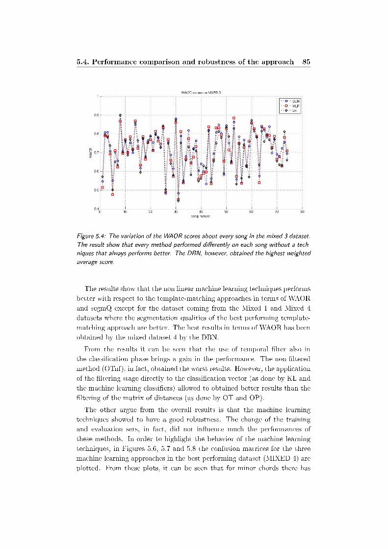
5.4. Performance comparison and robustness of the approach 85
Figure 5.4: The variation of the WAOR scores about every song in the mixed 3 dataset.
The result show that every method performed dierently on each song without a tech-
niques that always performs better. The DBN, however, obtained the highest weighted
average score.
The results show that the non linear machine learning techniques performs
better with respect to the template-matching approaches in terms of WAOR
and segmQ except for the dataset coming from the Mixed 1 and Mixed 4
datasets where the segmentation qualities of the best performing template-
matching approach are better. The best results in terms of WAOR has been
obtained by the mixed dataset 4 by the DBN.
From the results it can be seen that the use of temporal lter also in
the classication phase brings a gain in the performance. The non-ltered
method (OTnf), in fact, obtained the worst results. However, the application
of the ltering stage directly to the classication vector (as done by KL and
the machine learning classiers) allowed to obtained better results than the
ltering of the matrix of distances (as done by OT and OP).
The other argue from the overall results is that the machine learning
techniques showed to have a good robustness. The change of the training
and evaluation sets, in fact, did not inuence much the performances of
these methods. In order to highlight the behavior of the machine learning
techniques, in Figures 5.6, 5.7 and 5.8 the confusion matrices for the three
machine learning approaches in the best performing dataset (MIXED 4) are
plotted. From these plots, it can be seen that for minor chords there has

86 Chapter 5. Experimental results
Figure 5.5: The variation of the segmQ scores about every song in the mixed 3 dataset.
Like the WAOR case, the methods performed dierently on each song. Also in this
case the DBN obtained the highest weighted average score.
been the highest misclassication rate, while the most of major chords have
been successfully classied. The reason behind this behavior can be found
in the characteristics of the available dataset. As can be seen in gure 5.10,
the chord distribution on the training set is polarized towards major chords,
while minor chords are less present and this inuences the quality of the
learnt model.
As second test, we created other two datasets considering this time only
songs coming from the Beatles and Robbie Williams datasets alone. In
particular:
• a dataset containing 130 Beatles songs as training sets and 49 Bea-
tles songs as classication set. The training set size is 306327, the
evaluation set size is 131282;
• a dataset containing 45 Robbie Williams songs as training set and 20
Robbie Williams songs as classication. The training set size is 164712,
the evaluation set size is 70590.
The results of the experiment are shown in table 5.7.
The results show that the performances in these datasets are lower with
respect to the mixed datasets. However the performance decrease is common
to every method, and also the standard template-matching based techniques
suered from this problem.

5.4. Performance comparison and robustness of the approach 87
Figure 5.6: The confusion matrix for DBN with Gaussian input units on the Mixed
dataset MIXED 4. The gure shows how the dierent chords has been classied by
the DBN. A light color means a high number of elements, vice versa a dark colors
corresponds to low number of elements. If a square is white it means that all the
chords have been successfully classied.
OTnf OT OP KL LR MLP DBN
TB WAOR 0.612 0.632 0.680 0.640 0.675 0.689 0.689
TB segmQ 0.660 0.700 0.720 0.704 0.720 0.721 0.718
RW WAOR 0.636 0.650 0.678 0.652 0.685 0.689 0.698
RW segmQ 0.726 0.770 0.760 0.771 0.795 0.796 0.793
Table 5.7: The table shows the performances obtained by the dierent methods con-
sidering songs taken from the Beatles dataset (TB) and Robbie Williams dataset (RW)
highlighting the best performing method for each dataset.
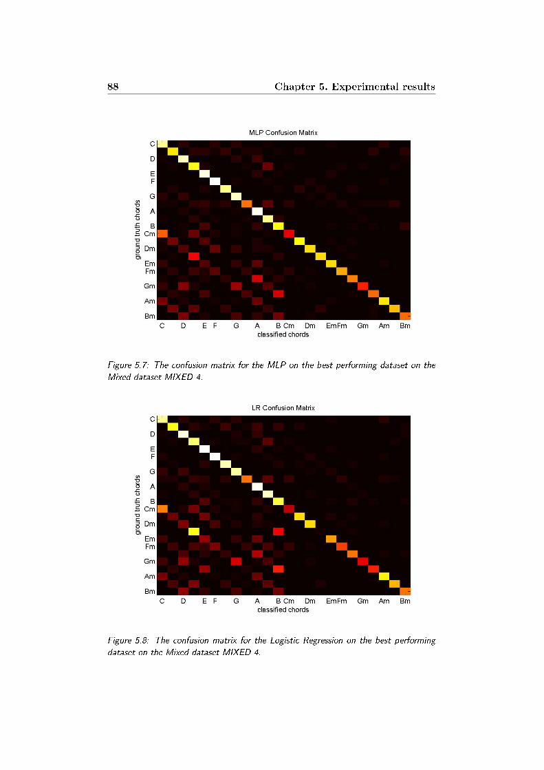
88 Chapter 5. Experimental results
Figure 5.7: The confusion matrix for the MLP on the best performing dataset on the
Mixed dataset MIXED 4.
Figure 5.8: The confusion matrix for the Logistic Regression on the best performing
dataset on the Mixed dataset MIXED 4.

5.4. Performance comparison and robustness of the approach 89
5.4.2 Experiment 2: change of Training Set cardinality
In the last experiment we tested the robustness of the approach considering
how the performances change varying the cardinality of the training set. For
the experiment, the method that resulted to be the best performing one in
the previous tests has been used for this experiment. In order to evaluate this
we changed the cardinality of the training set halving each time the number
of elements and we monitored the performance of the method. In particular
we used the DBN with Gaussian input units and the mixed dataset 4 used
for the previous tests evaluating the change of the WAOR score. The result
is shown in Figure 5.9.
Figure 5.9: The gure shows how the WAOR score is inuenced by the change of the
training set cardinality. Even when the number of elements is strongly reduced the
score is close to 0.6. The machine learning approach thus is robust to the training set
cardinality
The gure 5.9 shows that the performance of the method remains good
also when the number of elements in the training set become very small. In
particular, the results are still over the 60% when the 6.25% of the elements of
the original training set are considered. The results are close to the starting
point even when the elements of the dataset have been halved.
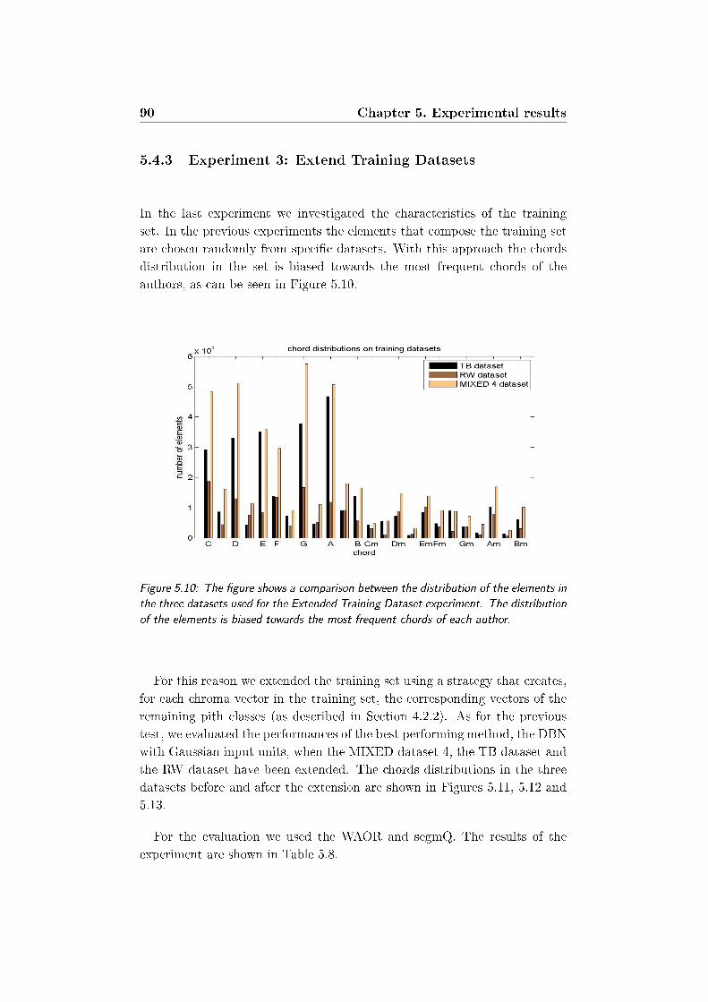
90 Chapter 5. Experimental results
5.4.3 Experiment 3: Extend Training Datasets
In the last experiment we investigated the characteristics of the training
set. In the previous experiments the elements that compose the training set
are chosen randomly from specic datasets. With this approach the chords
distribution in the set is biased towards the most frequent chords of the
authors, as can be seen in Figure 5.10.
Figure 5.10: The gure shows a comparison between the distribution of the elements in
the three datasets used for the Extended Training Dataset experiment. The distribution
of the elements is biased towards the most frequent chords of each author.
For this reason we extended the training set using a strategy that creates,
for each chroma vector in the training set, the corresponding vectors of the
remaining pith classes (as described in Section 4.2.2). As for the previous
test, we evaluated the performances of the best performing method, the DBN
with Gaussian input units, when the MIXED dataset 4, the TB dataset and
the RW dataset have been extended. The chords distributions in the three
datasets before and after the extension are shown in Figures 5.11, 5.12 and
5.13.
For the evaluation we used the WAOR and segmQ. The results of the
experiment are shown in Table 5.8.
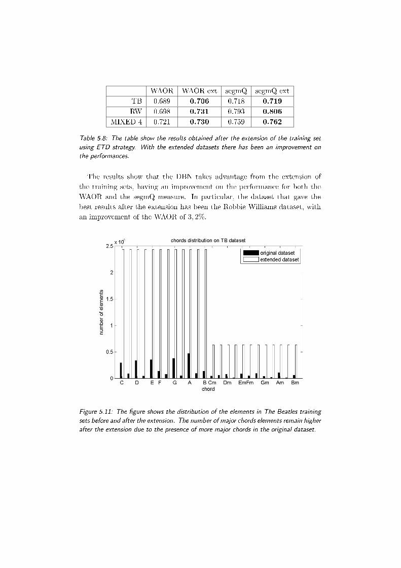
WAOR WAOR ext segmQ segmQ ext
TB 0.689 0.706 0.718 0.719
RW 0.698 0.731 0.793 0.806
MIXED 4 0.721 0.730 0.759 0.762
Table 5.8: The table show the results obtained after the extension of the training set
using ETD strategy. With the extended datasets there has been an improvement on
the performances.
The results show that the DBN takes advantage from the extension of
the training sets, having an improvement on the performance for both the
WAOR and the segmQ measure. In particular, the dataset that gave the
best results after the extension has been the Robbie Williams dataset, with
an improvement of the WAOR of 3, 2%.
Figure 5.11: The gure shows the distribution of the elements in The Beatles training
sets before and after the extension. The number of major chords elements remain higher
after the extension due to the presence of more major chords in the original dataset.
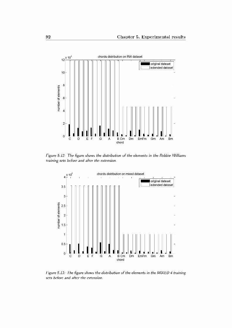
92 Chapter 5. Experimental results
Figure 5.12: The gure shows the distribution of the elements in the Robbie Williams
training sets before and after the extension.
Figure 5.13: The gure shows the distribution of the elements in the MIXED 4 training
sets before and after the extension.
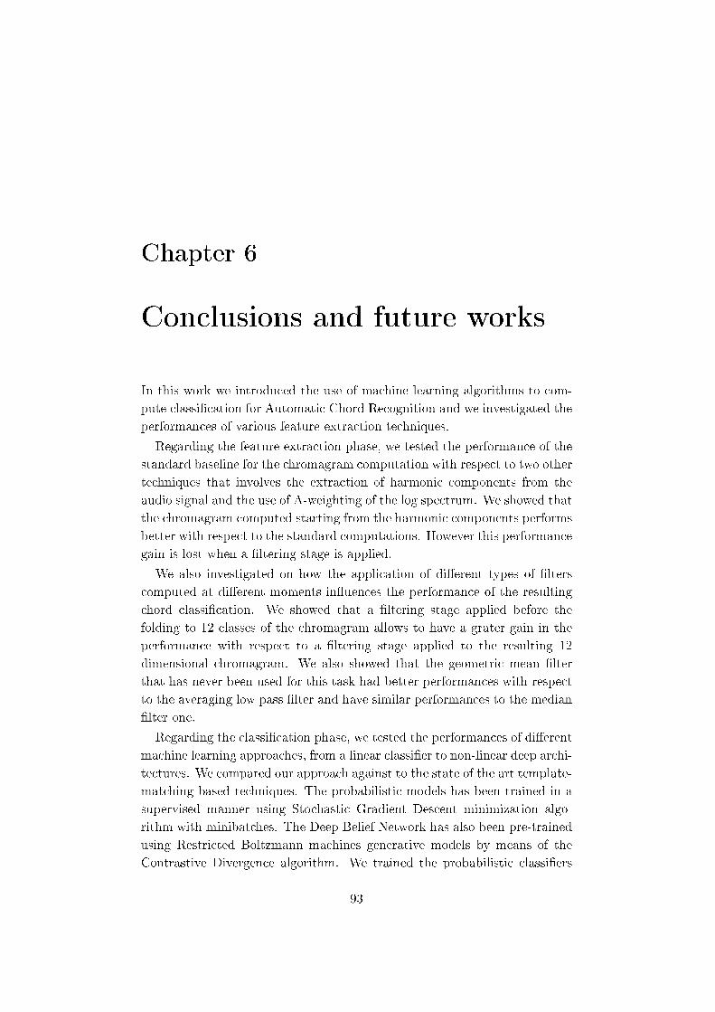
Chapter 6
Conclusions and future works
In this work we introduced the use of machine learning algorithms to com-
pute classication for Automatic Chord Recognition and we investigated the
performances of various feature extraction techniques.
Regarding the feature extraction phase, we tested the performance of the
standard baseline for the chromagram computation with respect to two other
techniques that involves the extraction of harmonic components from the
audio signal and the use of A-weighting of the log spectrum. We showed that
the chromagram computed starting from the harmonic components performs
better with respect to the standard computations. However this performance
gain is lost when a ltering stage is applied.
We also investigated on how the application of dierent types of lters
computed at dierent moments inuences the performance of the resulting
chord classication. We showed that a ltering stage applied before the
folding to 12 classes of the chromagram allows to have a grater gain in the
performance with respect to a ltering stage applied to the resulting 12
dimensional chromagram. We also showed that the geometric mean lter
that has never been used for this task had better performances with respect
to the averaging low pass lter and have similar performances to the median
lter one.
Regarding the classication phase, we tested the performances of dierent
machine learning approaches, from a linear classier to non-linear deep archi-
tectures. We compared our approach against to the state of the art template-
matching based techniques. The probabilistic models has been trained in a
supervised manner using Stochastic Gradient Descent minimization algo-
rithm with minibatches. The Deep Belief Network has also been pre-trained
using Restricted Boltzmann machines generative models by means of the
Contrastive Divergence algorithm. We trained the probabilistic classiers
93

94 Chapter 6. Conclusions and future works
on dierent datasets of high resolution chroma vectors obtained from ran-
dom songs chosen from the Beatles and Robbie Williams discography and
tested them on complete randomly chosen songs. We tried dierent types
of normalization of the input features nding out that the standardizations
allows to obtain better results. We showed that the use this kind of algo-
rithms allows to have better performances then the template-matching based
techniques, overcoming the problem of the creation and improvement of a
model of chords templates and the choice of a similarity measure. In partic-
ular Deep Learning techniques showed to have a great potential also in this
eld. Even if the main drawback of these methods is the dependence on the
creation of a training set, we showed that they are robust to the cardinality
and the type of training set. We also explored the possibility to extend the
training set creating articial observations of chroma vectors starting from
the available ones and showed that this technique can bring a gain to the
performances equalizing the number of observations of the chords elements
in the training set.
6.1 Future works
In order to have an improvement on the quality of the obtained chord tran-
scription, the successive step can be to include a machine learning classier,
like a Deep Belief Network, in a chord recognition framework that makes
use of probabilistic models of chord transitions. In particular, they can be
used as a replacement of the template-matching procedure that aims nding
the chord salience matrix. The probabilistic models of chord transitions, in
fact, allows to better exploit the temporal correlation between chords with
respect to the simple median ltering stage. However they are more complex
and they depend from a training stage or from an expert tuning.
The quality of the classication obtained with machine learning techniques
is still bound to the quality of the extracted feature, even if these methods
allows to reduce the confusion brought by the noise thanks to the non linear
processing of the input feature. For this reason the use of a better feature
than the chromagram can be further investigated. It can be extended to
add information from the bass note that can be used together with the
treble chromagram as input observation of the probabilistic classier. The
capability of extracting features of the DBN can be further explored and
other classiers at top of the network dierent from the Logistic Regressor
can be tested.
Even if the Deep Belief Networks obtained good performances in our tests,
a bottleneck to their performance gain is represented by the pre-training
stage of the Restricted Boltzmann Machines. These models are, in fact,
dicult to train and the choice of the incorrect parameters can make the
minimization algorithm diverge or can cause and increasing of overtting.
More sophisticated techniques for the training of the Restricted Boltzmann
Machines can be introduced. In particular, the momentum weights can be
added to the update rule of the Stochastic Gradient Descent algorithm and
weight decay can be introduced also for the pretraining stage.
For the netuning stage other minimization algorithms like Particle Swarm
Optimization can be tried instead of using the Stochastic Gradient Descent.
Finally, the netuning process of the Deep Belief Network can be also done
in a partially supervised manner instead of a totally supervised fashion.

96 Chapter 6. Conclusions and future works

Bibliography
[1] Itamar Arel, Derek C. Rose, and Thomas P. Karnowski. Deep machine
learning - a new frontier in articial intelligence research. Comp. Intell.
Mag., 5:1318, 2010.
[2] Di Giorgi B., Zanoni M., Sarti A., and Tubaro S. Automatic chord recog-
nition based on the probabilistic modeling of diatonic modal harmony.
In In proceedings of the 8th international workshop on multidimensional
(nD) systems - nDS13, pages 126131, Erlangen, Germany, September
2013.
[3] Juan P Bello and Jeremy Pickens. A robust mid-level representation for
harmonic content in music signals. In In prococeedings of ISMIR, pages
304311, 2005.
[4] Yoshua Bengio. Greedy layer-wise training of deep networks. In In
proseedings of NIPS, 2007.
[5] Yoshua Bengio. Learning deep architectures for ai. Foundations and
Trends in Machine Learning, 2:1127, 2009.
[6] James Bergstra, Olivier Breuleux, Frédéric Bastien, Pascal Lamblin,
Razvan Pascanu, Guillaume Desjardins, Joseph Turian, David Warde-
Farley, and Yoshua Bengio. Theano: a CPU and GPU math expression
compiler. In Proceedings of the Python for Scientic Computing Con-
ference (SciPy), 2010.
[7] Judith C Brown. Calculation of a constant q spectral transform. The
Journal of the Acoustical Society of America, 89:425, 1991.
[8] Ruofeng Chen, Weibin Shen, Ajay Srinivasamurthy, and Parag Chordia.
Chord recognition using duration-explicit hidden markov models, 2012.
[9] Matthew EP Davies and Mark D Plumbley. A spectral dierence ap-
proach to downbeat extraction in musical audio. In Proc. EUSIPCO.
Citeseer, 2006.
97

98 BIBLIOGRAPHY
[10] Takuya Fujishima. Realtime chord recognition of musical sound: a
system using common lisp music. In In proceedings of international
computer music association (ICMC), 1999, pages 464467, 1999.
[11] Bruno Di Giorgi. Automatic chord recognition based on the probabilistic
modeling of diatonic modal harmony. Master's thesis, Politecnico di
Milano, 2013.
[12] Glaziryn. Audio chord estimation using chroma reduced spectrogram
and self-similarity. In in Proceedings of the Music Information Retrieval
Evaluation Exchange (MIREX), 2012.
[13] Glaziryn. Mid-level features for audio chord estimation using stacked
denoising autoencoders. 2013.
[14] Xavier Glorot and Yoshua Bengio. Understanding the diculty of train-
ing deep feedforward neural networks. In In Proceedings of the Interna-
tional Conference on Articial Intelligence and Statistics, 2010.
[15] Emilia Gómez Gutiérrez. Tonal description of music audio signals. PhD
thesis, Univeritat Pompeu Fabra, 2006.
[16] Christopher Harte, Mark Sandler, Samer Abdallah, and Emilia Gómez.
Symbolic representation of musical chords: A proposed syntax for text
annotations. In Proceedings of the International Conference on Music
Information Retrieval (ISMIR), pages 6671, 2005.
[17] Christopher A Harte and Mark B Sandler. Automatic chord identi-
cation using a quantised chromagram. In Proceedings of the Audio
Engineering Society, 2005.
[18] Trevor Hastie, Robert Tibshirani, and Jerome Friedman. The Elements
of Statistical Learning. Springer, 2001.
[19] Georey Hinton. Products of experts. In In proceedings of the Ninth
International Conference of Articial Neural Networks, 1999.
[20] Georey Hinton. A practical guide to training restricted boltzmann
machines. In Neural Networks: Tricks of the Trade (2nd ed.). Springer,
2012.
[21] Georey Hinton, Simon Osindero, and Yee-Whye Teh. A fast learning
algorithm for deep belief nets. Neural Computation, 18:15271554, 2006.

BIBLIOGRAPHY 99
[22] Bello Humphrey. Rethinking automatic chord recognition with convo-
lutional neural networks. In In proceedings of international conference
on machine learning and applications, 2012.
[23] Eric J. Humphrey, Juan Pablo Bello, and Yann LeCun. Moving beyond
feature design: Deep architectures and automatic feature learning in
music informatics. In ISMIR, pages 403408, 2012.
[24] Omologo Khadkevich. Time-frequency reassigned features for automatic
chord recognition. In in Proceedings of the IEEE International Confer-
ence on Acoustics, Speech and Signal Processing (ICASSP), 2011.
[25] Anssi P Klapuri, Antti J Eronen, and Jaakko T Astola. Analysis of
the meter of acoustic musical signals. Audio, Speech, and Language
Processing, IEEE Transactions on, 14(1):342355, 2006.
[26] Mark Levine. The Jazz Piano Book. 1989.
[27] Matthias Mauch. Automatic Chord Transcription from Audio Using
Computational Models of Musical Context. PhD thesis, Queen Mary
University of London, 2010.
[28] Matthias Mauch and Simon Dixon. Simultaneous estimation of chords
and musical context from audio. Audio, Speech, and Language Process-
ing, IEEE Transactions on, 18(6):12801289, 2010.
[29] Yizhao Ni, Matt McVicar, Raul Santos-Rodriguez, and Tijl De Bie.
An end-to-end machine learning system for harmonic analysis of mu-
sic. Audio, Speech, and Language Processing, IEEE Transactions on,
20(6):17711783, 2012.
[30] Ono, Miyamoto, Le Roux, Kameoka, and Sagayama. Separation of a
monoaural audio signal into harmonic/percussive components by com-
plementary diusion on spectrogram. In in Proceedings of EUSIPCO,
2008.
[31] L. Oudre, Y. Grenier, and C. Fevotte. Chord recognition by tting
rescaled chroma vectors. IEEE transaction on Audio, Speech and Image
processing, 19:22222223, 2011.
[32] Laurent Oudre, Yves Grenier, and Cédric Févotte. Template-based
chord recognition: Inuence of the chord types. In Proceedings of the
10th International Society for Music Information Retrieval Conference
(ISMIR 2009), pages 153158, 2009.

100 BIBLIOGRAPHY
[33] Laurent Oudre, Yves Grenier, and Cédric Févotte. A probabilistic
template-based chord recognition method. In Proceedings of the 11th
International Society for Music Information Retrieval Conference (IS-
MIR 2010), 2010.
[34] Hélene Papadopoulos and Georoy Peeters. Simultaneous estimation
of chord progression and downbeats from an audio le. In Acoustics,
Speech and Signal Processing, 2008. ICASSP 2008. IEEE International
Conference on, pages 121124. IEEE, 2008.
[35] Raul Rojas. Neural Networks - A Systematic Introduction. SSpringer-
Verlag, 1996.
[36] Luigi Rossi. Teoria Musicale. Casa Musicale Edizione Carrara, 1977.
[37] Erik M. Schmidt and Youngmoo E. Kim. Learning emotion-based acous-
tic features with deep belief networks. In In proceedings of WASPAA,
2011.
[38] John A Sloboda. Music structure and emotional response: Some em-
pirical ndings. Psychology of music, 19(2):110120, 1991.
[39] William A. Yost. Pitch perception. Attention, Perception and Psy-
chophysics, 8:17011715, 2009.


![CHORD CATALOGS AND ESTRADA CLASSES: PARTIALLY … · 2017-03-22 · Geometric Logic of Concepts, Theory, and Performance [Maz02]. The cen-tral role of group actions and categories](https://static.fdocumenti.com/doc/165x107/5edb2ec2d96bc859bd1d6941/chord-catalogs-and-estrada-classes-partially-2017-03-22-geometric-logic-of-concepts.jpg)