A Refined Zigzag Beam Theory for Composite and Sandwich Beams

Alexander Tessler

Structural Mechanics and Concepts Branch – NASA Langley Research Center Mail Stop 190, Hampton, Virginia, 23681 - 2199, U.S.A.

Marco Di Sciuva, Marco Gherlone1

Department of Aeronautics and Space Engineering – Politecnico di Torino Corso Duca degli Abruzzi 24

10129, Torino, Italy

ABSTRACT

A new refined theory for laminated composite and sandwich beams that contains the kinematics of the

Timoshenko Beam Theory as a proper baseline subset is presented. This variationally consistent

theory is derived from the virtual work principle and employs a novel piecewise linear zigzag

function that provides a more realistic representation of the deformation states of transverse-shear

flexible beams than other similar theories. This new zigzag function is unique in that it vanishes at the

top and bottom bounding surfaces of a beam. The formulation does not enforce continuity of the

transverse shear stress across the beam’s cross-section, yet is robust. Two major shortcomings that are

inherent in the previous zigzag theories, shear-force inconsistency and difficulties in simulating

clamped boundary conditions, and that have greatly limited the utility of these previous theories are

discussed in detail. An approach that has successfully resolved these shortcomings is presented

herein. Exact solutions for simply supported and cantilevered beams subjected to static loads are

derived and the improved modelling capability of the new “zigzag” beam theory is demonstrated. In

2

particular, extensive results for thick beams with highly heterogeneous material lay-ups are discussed

and compared with corresponding results obtained from elasticity solutions, two other “zigzag”

theories, and high-fidelity finite element analyses. Comparisons with the baseline Timoshenko Beam

Theory are also presented. The comparisons clearly show the improved accuracy of the new, refined

“zigzag” theory presented herein over similar existing theories. This new theory can be readily

extended to plate and shell structures, and should be useful for obtaining relatively low-cost, accurate

estimates of structural response needed to design an important class of high-performance aerospace

structures.

KEYWORDS

Timoshenko beam theory, Zigzag kinematics, Shear deformation, Composite beams, Sandwich

beams, Virtual work principle

1 Author to whom correspondence should be sent: Tel. +39-0115646817, FAX +39-0115646899, EMAIL marco.gherlone@polito.it

3

NOMENCLATURE

, 2 ,A h L = beam’s cross-sectional area, depth, and span

( )2 kh = thickness of the k -th layer

,q F = transverse pressure loading [force/length] and tip shear force

( ),xr zrT T = axial and shear tractions prescribed at the ends of beam

( , )rx r a b=

( )( ) ( ),k kx zu u = axial and transverse components of the displacement vector in

the k -th layer

( ), , ,u wθ ψ = kinematic variables of zigzag theory

( )kφ = zigzag function

( )( ) ( ),k kx xzε γ = axial and transverse shear strain in the k -th layer

( )( ) ( ),k kx xzσ τ = axial and transverse shear stress in the k -th layer

( )( ) ( ),k kx xzE G = axial and shear modulus of the k -th layer

Aλ , 0λ = penalty factors

( )kξ = local ( k -th layer) thickness coordinate

( )ku = normalized axial displacement along the interface between

the k -th and ( 1)k + layers

( ), , , ,x x xN M M V Vφ φ = stress resultants of the refined zigzag beam theory

11A , ijB , ijD , and ijQλ = constitutive stiffness coefficients of the refined zigzag beam

theory

4

1. INTRODUCTION

Performance and weight advantages of advanced composite materials have led to their sustained

and increased application to military and civilian aircraft, aerospace vehicles, naval and civil

structures. To design efficient and reliable composite structures, improved analytical and

computational methods that accurately incorporate principal non-classical effects are necessary. In

relatively thick and/or heterogeneous beams, shear deformation may influence, to a significant

degree, such design-significant response quantities as the normal stresses, deflection, vibration

modes, and natural frequencies. The inherent assumptions of classical deformation theories generally

render such theories less than adequate for application to advanced composites. This shortcoming is

particularly manifested in relatively thick structures with material layers that exhibit large differences

in the transverse shear properties, often leading to non-conservative predictions for deformation,

stresses, and natural frequencies. It is further noted that, in these classical shear deformation models,

transverse shear stresses fail to satisfy equilibrium conditions at the layer interfaces.

The two key assumptions of Bernoulli-Euler beam (known as the Kirchhoff-Love hypotheses in

plates and shells) are those of zero transverse shear strain and non-deformable transverse normal – the

assumptions that are fully consistent for the bending of very slender beams that exhibit negligibly

small shear deformations. The bending deformation may thus be defined in terms of a single

deflection variable. Here Hooke’s law only leads to a zero transverse shear stress. Instead, a beam

equilibrium equation is used to obtain the shear force from which an average shear stress is computed.

Timoshenko1 introduced an additional kinematic variable, the bending rotation, to account for shear

deformation in an average sense while retaining the non-deformable normal assumption. This

improvement over the classical beam theory allows the transverse shear stress to be obtained from

Hooke’s law, and extends the range of applicability to thick beams.

Timoshenko beam theory, and analogous shear-deformation theories for plate and shell structures,

5

has been widely used in structural analysis of homogeneous and composite beam-type structures. The

theory produces inadequate predictions, however, when applied to relatively thick composite

laminates composed of material layers that have highly dissimilar stiffness characteristics. Even with

a judiciously chosen shear correction factor, which is dependent on the stacking sequence,

Timoshenko theory tends to underestimate, often substantially, the axial stress on the top and bottom

surfaces. Moreover, along layer interfaces, the transverse shear stress often exhibits excessively

erroneous discontinuities. The reason for these difficulties might be traced to a higher complexity of

the ‘true’ displacement field across a highly heterogeneous cross-section. Clearly, the linear through-

thickness displacement assumption for the axial displacement is the main shortcoming of Timoshenko

theory when the modelling of complex material systems is undertaken.

Higher-order terms, with respect to the thickness coordinate, have been added to the in-plane

displacements and, in some cases, to the transverse displacement. This leads to the so-called higher-

order theories that are also commonly known as equivalent single-layer theories2. While notable

response improvements have been achieved with several of such theories, they generally fall short as

far as predicting correct shear and axial stress behaviour in highly heterogeneous lay-ups in

moderately thick laminates and high-frequency dynamics.

Departing from the equivalent single-layer modelling assumptions, layer-wise theories assume that

the behaviour of a laminate is due to an assembly of the individual layers whose kinematic fields are

independently described while satisfying certain physical continuity constraints2. The increased

kinematic freedom provided by the layer-wise schemes enable the enforcement of the interlaminar

stress continuity conditions and the modelling of the zigzag displacement through a laminate

thickness. The major drawback of such theories, however, is that the number of kinematic variables is

dependent on the number of layers; thus, for thick laminates with a large number of plies, a great

number of variables results, making such approaches computationally unattractive. Notable early

contributions to layer-wise schemes are those due to Ambartsumian3 and Sun and Whitney4. While

providing relatively accurate approximations, these theories possess a large number of variables and

6

are particularly cumbersome to implement within a displacement-based finite element method5.

The so-called zigzag theories constitute a special sub-class of layer-wise theories. They assume a

zigzag pattern for the in-plane displacements and enforce the continuity of the shear stresses across

the entire laminate thickness. They give rise to bending theories based on the same number of

kinematic variables regardless of the number of layers in a laminate. Thus, the early efforts of Di

Sciuva6-8 and Murakami9 employed zigzag-like displacement fields that satisfy a priori the transverse

shear stress and displacement continuity conditions at the layer interfaces while keeping the number

of kinematic variables independent of the number of layers. Di Sciuva10-11 also demonstrated that

such models are well-suited for finite element approximations.

In Di Sciuva’s earlier efforts6-7, a form of shear deformation theory is augmented by adding a

piecewise linear (“zigzag”) function to the in-plane displacement. To retain only the kinematic

variables of the classical theory, a constant shear stress is enforced across the entire laminate

thickness. This procedure led to the desired enhancement in the axial displacement and

simultaneously achieved the shear stress continuity along layer interfaces. Furthermore, for

homogeneous cross-sections the zigzag shape function vanishes identically, thus resorting back to a

shear deformation theory. Di Sciuva12-13 also introduced further enhancements to the zigzag model by

adding to a zigzag function a cubic in-plane displacement. The Di Sciuva theories require C1–

continuous shape functions for formulating suitable finite elements. Such approximation schemes are

significantly less attractive, especially for plate and shell finite elements, than the C0–continuous

displacement interpolations associated with Timoshenko-type theories.

Exploring the new linear14 and cubic15 zigzag beam models with a view on C0–continuous finite

elements, Averill modified the Di Sciuva approach by starting with Timoshenko theory, adding an

additional kinematic variable associated with a zigzag function, and by introducing an ad hoc penalty

term in the variational principle. The penalty term serves to enforce the continuity of transverse shear

stress across the cross-section in a limiting sense.

Di Sciuva’s theory runs into theoretical difficulties in an attempt to interpret the physical

7

significance of the shear stress associated with the theory. The difficulty is especially evident at the

clamped support, where the cross-sectional area integral of the shear stress, obtained from constitutive

relations, does not correspond to the total shear force. Thus, the correct shear force and the average

shear stress can be determined from an equilibrium equation relating the shear force to the derivative

of the bending moment, as in Bernoulli-Euler theory. Averill’s theory also suffers from its inability to

model correctly a clamped boundary condition, where it predicts erroneously that the transverse shear

stress and the corresponding resultant force vanish. To alleviate this anomaly, Averill proposed a

boundary condition compromise at the expense of variational consistency of the theory, in which a

kinematic variable representing the amplitude of the zigzag displacement is left out of the

variationally required boundary condition. Consequently, extensive analytic and numerical studies

that have been conducted primarily focused on beams and plates with simply supported boundaries6-

7,12-15. Recently, a zigzag plate analysis was discussed for clamped plates16; however, no results were

presented for the shear stresses along the clamped edges.

Scrutiny of the zigzag theories discussed herein has revealed some serious shortcomings. The aim

of the present study is to present a new refined zigzag theory that is free of these shortcomings and

amenable to finite element implementation. In particular, the present paper discusses a new refined

zigzag beam theory of Tessler, Di Sciuva and Gherlone17,18 that is consistently derived from the virtual

work principle, by refining the ideas of Timoshenko, Di Sciuva, and Averill. The key attributes of the

present theory are, first, the proposed zigzag function vanishes at the top and bottom surfaces of the

beam and does not require full shear-stress continuity across the laminated-beam depth. Second, all

boundary conditions, including the fully clamped condition, can be modelled adequately. And third,

the theory requires only C0-continuous kinematics for finite element modelling, as do elements based

on the theories of Timoshenko1, Mindlin19, and Reissner20. This latter attribute lends itself to

developing computationally efficient and robust beam, plate, and shell finite elements. Overall, the

theory appears as a natural extension of Timoshenko theory to laminated composite beams, and it is

devoid of the drawbacks of the zigzag theories discussed previously.

8

In the remainder of the paper, the concept of zigzag kinematic assumptions is first described.

Then the original zigzag schemes of Di Sciuva and Averill are elaborated in detail, and their

deficiencies with respect to the transverse shear properties and clamped boundary conditions are

highlighted. A unique zigzag function is then introduced to formulate the basis for the refined zigzag

theory, giving rise to the transverse shear stress that has a piecewise constant distribution across the

laminate thickness. As an added explanation of the underlying reasons for the drawbacks of Averill’s

formulation, a penalized form of the constitutive equations is introduced within the present theory.

The equations of equilibrium and associated boundary conditions are then derived from the virtual

work principle. Finally, the refined zigzag theory is assessed quantitatively by way of exact solutions

for simply supported and cantilevered composite and sandwich beams. Thick beams composed of

highly heterogeneous material lay-ups are considered. Comparisons are made with several beam

theories, exact elasticity solutions, and results obtained with high-fidelity, two-dimensional elasticity

finite element models.

This paper is an enhanced version of the article18 presented at the VI International Symposium

on Advanced Composites and Applications for the New Millennium, held in Corfù, Greece, in May

2007.

2. CONCEPT OF ZIGZAG KINEMATICS

The response of heterogeneous, anisotropic laminated beams exhibiting the bending, shear and

axial deformations is generally manifested by a zigzag-like through-thickness displacement field.

Here the axial displacements are dominant, mainly in thick and/or heterogeneous beams, in their

influence on the bending strain and stress. The cross-section of the deformed beam tends to distort

according to a piecewise C0-continuous pattern, having discontinuous thickness-direction derivatives

along the material layer interfaces. Within the individual material layers, the displacement

distributions are generally nonlinear and sufficiently smooth. Such observations, based on exact

9

elasticity solutions (e.g., Pagano21), prompted Di Sciuva7 to add a zigzag kinematic term to a first-

order shear deformation theory in which shearing angles appear as independent variables. Following

Di Sciuva’s work, Averill14 proposed a similar zigzag enhancement for application to beam bending

analysis of composite laminates using the standard form of Timoshenko theory in which the bending

rotation is represented by an independent variable appearing in the axial displacement expansion. In

what follows, the essential aspects of Di Sciuva and Averill zigzag models are examined in order to

set the stage for the new refined zigzag bending theory. The theoretical anomalies encountered by

these earlier zigzag models are discussed in sufficient detail.

Consider a narrow beam with the cross sectional area A. The beam is made of N orthotropic

material layers that are perfectly bonded to each other and are parallel to the x axis. For the sake of

the present discussion, only planar deformations are considered under the static loading which

includes a distributed transverse pressure q(x) (units of force/length) and the prescribed axial (Txa, Txb)

and shear (Tza, Tzb) tractions at the two reference cross sections x=xa and xb (refer to Figure 1).

Figure 1. Beam subjected to transverse loading and end tractions.

For any material point within the k-th layer, the displacement vector, which is general enough to

describe the kinematics of the Di Sciuva, Averill, and the present refined zigzag theory, is expressed

herein as

10

( ) ( )

( )

( , ) ( ) ( ) ( ) ( )

( , ) ( )

k kxk

z

u x z u x z x z x

u x z w x

θ φ ψ= + +

= (1)

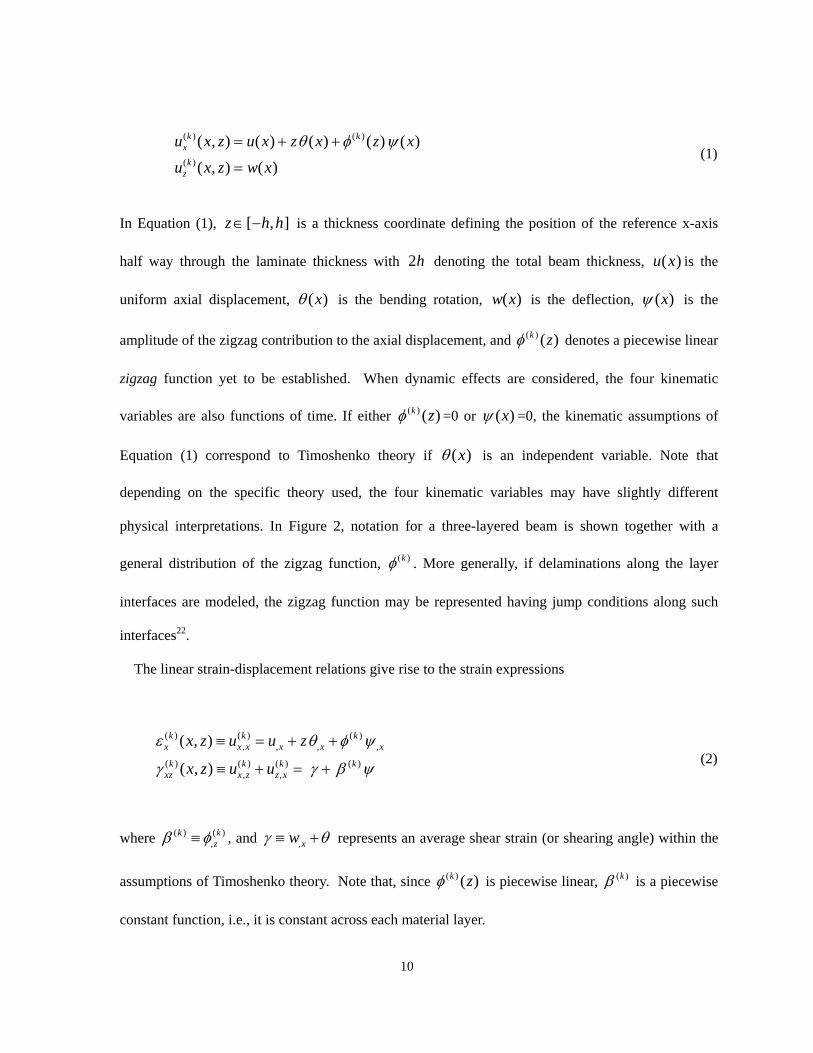
In Equation (1), [ , ]z h h∈ − is a thickness coordinate defining the position of the reference x-axis

half way through the laminate thickness with 2h denoting the total beam thickness, ( )u x is the

uniform axial displacement, ( )xθ is the bending rotation, ( )w x is the deflection, ( )xψ is the

amplitude of the zigzag contribution to the axial displacement, and ( ) ( )k zφ denotes a piecewise linear

zigzag function yet to be established. When dynamic effects are considered, the four kinematic

variables are also functions of time. If either ( ) ( )k zφ =0 or ( )xψ =0, the kinematic assumptions of

Equation (1) correspond to Timoshenko theory if ( )xθ is an independent variable. Note that

depending on the specific theory used, the four kinematic variables may have slightly different

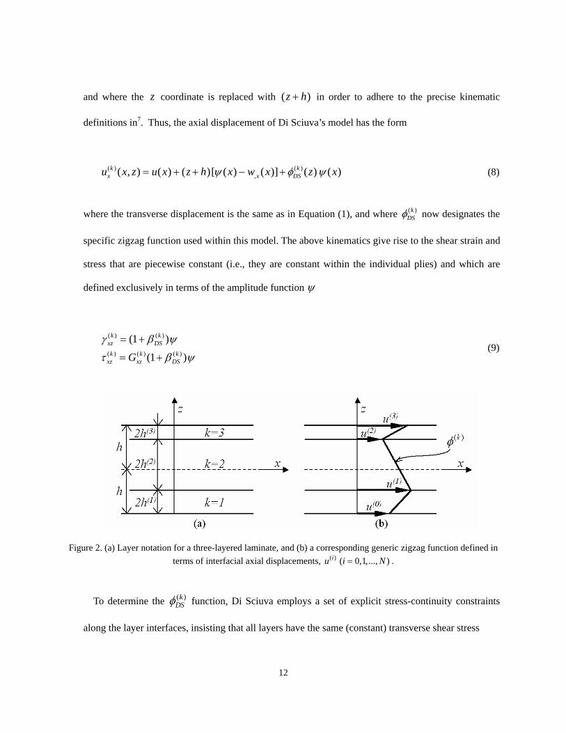
physical interpretations. In Figure 2, notation for a three-layered beam is shown together with a

general distribution of the zigzag function, ( )kφ . More generally, if delaminations along the layer

interfaces are modeled, the zigzag function may be represented having jump conditions along such

interfaces22.

The linear strain-displacement relations give rise to the strain expressions

( ) ( ) ( ), , , ,

( ) ( ) ( ) ( ), ,

( , )

( , )

k k kx x x x x x

k k k kxz x z z x

x z u u z

x z u u

ε θ φ ψ

γ γ β ψ

≡ = + +

≡ + = + (2)

where ( ) ( ),

k kzβ φ≡ , and ,xwγ θ≡ + represents an average shear strain (or shearing angle) within the

assumptions of Timoshenko theory. Note that, since ( ) ( )k zφ is piecewise linear, ( )kβ is a piecewise

constant function, i.e., it is constant across each material layer.

11

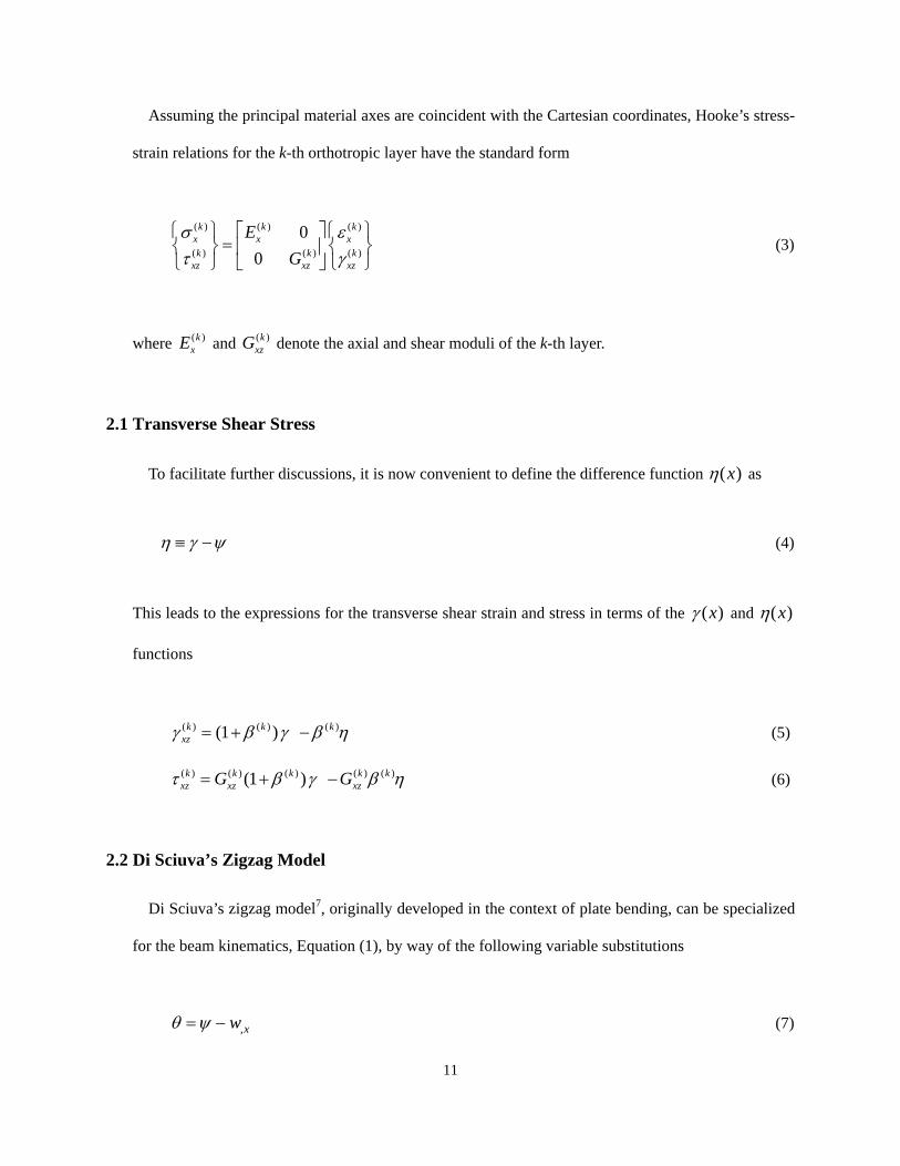
Assuming the principal material axes are coincident with the Cartesian coordinates, Hooke’s stress-

strain relations for the k-th orthotropic layer have the standard form

( ) ( ) ( )

( ) ( ) ( )

00

k k kx x xk k k

xz xz xz

EG

σ ετ γ⎧ ⎫ ⎡ ⎤ ⎧ ⎫

=⎨ ⎬ ⎨ ⎬⎢ ⎥⎩ ⎭ ⎣ ⎦ ⎩ ⎭

(3)

where ( )kxE and ( )k

xzG denote the axial and shear moduli of the k-th layer.

2.1 Transverse Shear Stress

To facilitate further discussions, it is now convenient to define the difference function ( )xη as

η γ ψ≡ − (4)

This leads to the expressions for the transverse shear strain and stress in terms of the ( )xγ and ( )xη

functions

( ) ( ) ( )(1 )k k kxzγ β γ β η= + − (5)

( ) ( ) ( ) ( ) ( )(1 )k k k k kxz xz xzG Gτ β γ β η= + − (6)

2.2 Di Sciuva’s Zigzag Model

Di Sciuva’s zigzag model7, originally developed in the context of plate bending, can be specialized

for the beam kinematics, Equation (1), by way of the following variable substitutions

,xwθ ψ= − (7)

12

and where the z coordinate is replaced with ( )z h+ in order to adhere to the precise kinematic

definitions in7. Thus, the axial displacement of Di Sciuva’s model has the form

( ) ( ),( , ) ( ) ( )[ ( ) ( )] ( ) ( )k k

x x DSu x z u x z h x w x z xψ φ ψ= + + − + (8)

where the transverse displacement is the same as in Equation (1), and where ( )kDSφ now designates the

specific zigzag function used within this model. The above kinematics give rise to the shear strain and

stress that are piecewise constant (i.e., they are constant within the individual plies) and which are

defined exclusively in terms of the amplitude function ψ

( ) ( )

( ) ( ) ( )

(1 )

(1 )

k kxz DSk k k

xz xz DSG

γ β ψ

τ β ψ

= +

= + (9)

Figure 2. (a) Layer notation for a three-layered laminate, and (b) a corresponding generic zigzag function defined in terms of interfacial axial displacements, ( ) ( 0,1,..., )iu i N= .

To determine the ( )k

DSφ function, Di Sciuva employs a set of explicit stress-continuity constraints

along the layer interfaces, insisting that all layers have the same (constant) transverse shear stress

13

( ) ( 1) , 1,..., 1k kxz xz k Nτ τ += = − (10)

Since the above equations impose only 1N − constraints, and there are 1N + interfacial

displacements ( ) ( 0,1,..., )iu i N= which define ( )kDSφ , the zigzag function is set to vanish across the

entire bottom layer ( 1k = , refer to Figure 3(a)). More generally, it is straightforward to select any

layer in which a zigzag function may vanish22. Henceforth, determining a zigzag function by way of

zeroing out (or fixing) a single layer contribution will be referred to as a fixed-layer zigzag function

method.

Figure 3. (a) Di Sciuva7 and (b) Averill14 zigzag functions.

The resulting transverse shear stress is uniform through the thickness. If the first layer ( 1k = ) is

fixed in the definition of the zigzag function ( (1) (1) 0DS DSφ β= = ), as depicted in Figure 3(a), then from

Equation (9), the definition of ψ as the shear strain in the first layer becomes evident

(1)xzψ γ= (11)

and, taking into account Equation (11), the shear stress in all layers simply equals the stress in the first

14

layer

( ) (1) (1) ( 1,..., )kxz xz xzG k Nτ γ= = (12)

As seen from Equation (12), all shear stresses in this model depend on the shear modulus and shear

strain in the first layer; hence the validity of this result is questionable. More generally, the shear

stress continuity enforcement, Equation (10), leads to the lack of invariance with respect to the choice

of the fixed-layer definition of the zigzag function. The shear modulus of the fixed layer thus serves

as a single weighting coefficient for the entire shear strain energy, thus producing a bias toward the

shear stiffness of the fixed layer. In contrast, ( )kDSφ depends on all shear moduli, ( )k

xzG , and ply

thicknesses, ( )2 kh . Its key property is that it vanishes identically when the transverse shear properties

are homogeneous, in which case the theory reverts to the underlying shear-deformation theory. The

improvements contributed toward solutions for the axial strain, stress, and energy due to the ( )kDSφ ψ

term in Equation (1) are particularly appreciable for thick and highly heterogeneous laminates (refer

to Section 4).

Di Sciuva’s theory runs into further theoretical difficulties in an attempt to interpret the

consequences of the shear stress continuity constraints and the resulting uniform shear stress. On the

one hand, the correct shear force ( )xV x can be determined from the well-established shear-moment

relationship

,x x xV M= (13)

which has its origin in the virtual work principle. On the other hand, the shear stress in Equation (12),

when integrated over the cross-section, does not yield the correct shear force

15

( ) (1)kx xz xz

A

V dA Aτ τ≠ =∫ (14)

A related theoretical anomaly is immediately apparent at a clamped support condition for which the

variationally consistent displacement boundary conditions are given as

, 0xu w w ψ= = = = (15)

Because 0ψ = is required at the clamped end, the corresponding transverse shear strain and stress

defined in Equation (9) vanish identically. In contrast, a non vanishing average shear stress

/xz xV Aτ = at a clamped end is computed from the shear force obtained from the equilibrium

equation given by Equation (13).

From the perspective of finite element approximations appropriate for this theory, ( )w x needs to

be at least C1 continuous, since the axial strain is proportional to the second derivative of ( )w x . This

requirement yields an added impediment for the approximating functions, particularly for developing

efficient plate and shell elements based on this class of theory. It has been shown, however, that C 0

continuous kinematic approximations, usually associated with shear deformation theories of

Timoshenko1, Mindlin19 and Reissner20, result in simpler, computationally more efficient, and better

performing finite elements than comparable elements based on C1 continuous interpolations23. It is

this aspect that motivated Averill14 to introduce a zigzag model based upon the standard form of

Timoshenko theory that uses an independent bending rotation variable in the axial displacement

expansion.

2.3 Averill’s Zigzag Model

Averill14 proposed a penalty formulation, herein referred to as a Penalized Zigzag (PZ) theory,

16

using the standard Timoshenko kinematics as an underlying theory. Consistent with the definition of

the fixed zigzag function within the second layer ( 2k = ), the axial displacement of the PZ theory

may be expressed as

( ) (1) ( )( , ) ( ) ( 2 ) ( ) ( ) ( )k kx Au x z u x z h h x z xθ φ ψ= + + − + (16)

where within this specific example, ( )xθ represents the rotation of the second layer, (2),x zu θ= , and

( )kAφ denotes Averill’s zigzag function depicted in Figure 3(b).

Shear stress continuity conditions, Equation (10), are enforced explicitly only on the first part of

the shear stress, Equation (6), by setting ( ) ( )(1 )k kA xzG G β≡ + to be constant across the material

layers. Herein, since the second layer is fixed in the sense of the zigzag function, (2) (2) 0A Aφ β= = ,

thus (2)A xzG G= and the shear stress reduces to

( ) (2) ( ) ( ) ( 1,..., )k k kxz xz xz AG G k Nτ γ β η= − = (17)

where (2)xzγ γ= defines the shear strain in the second (or fixed) layer. Further, the second term in

Equation (17) is set to diminish to zero in a limiting sense by letting

0η γ ψ≡ − → (18)

with the aid of a penalty constraint term which is added to the strain energy

2

2b

a

xAx

I dxλλ η≡ ∫ (19)

17

In the above definition, Aλ represents a penalty factor (units of force) which is set to a large value

( Aλ →∞ ) to ensure the validity of Equation (18). The subscript ( )A⋅ denotes quantities

corresponding to Averill’s model. Under these conditions, the shear stresses are uniform only in a

limiting sense

( ) ( 1) (2) ( 1,..., 1)k kxz xz xzG k Nτ τ γ+→ → = − (20)

For this theory, the shear force derived from the virtual work principle is given as

( ) ( )kx xz A

A

V dA xτ λ η≡ +∫ (21)

When the penalty parameter Aλ →∞ , ( )1 0AOη λ= → and the term ( )A xλ η takes on a finite

value; thus, the shear force in Equation (21), which is derived from the virtual work principle, does

not correspond to the cross-sectional integral of the shear stress. Whereas Averill’s model results in a

four-variable theory and C0 continuous kinematics suitable for efficient finite element interpolations,

the theory appears to possess some theoretical anomalies. As in Di Sciuva’s model, there is the fixed-

layer anomaly manifesting itself with a bias toward the shear properties of the fixed layer. This means

that the methodology lacks invariance with respect to the choice of the fixed layer. Moreover, the

theory breaks down at the clamped end. Because the clamped boundary conditions require the

vanishing of the four kinematic variables

0u w θ ψ= = = = (22)

and the penalization condition Equation (18) yields an additional constraint , 0xw → , the following

erroneous conditions for the shear strain and stress at the clamped end result

18

( )( ) ( )@clamped

support, 0k k

xz xzγ τ → (23)

Averill recognized the above anomaly and proposed to avoid prescribing boundary conditions on the

ψ variable, thus violating the theory’s variational requirements.

The theoretical difficulties just discussed, associated with the Di Sciuva7 and Averill14 zigzag

theories, serve as motivation for developing a consistent shear deformable zigzag theory that

incorporates the proper zigzag kinematics which is devoid of the above mentioned anomalies. In what

follows, the mathematical foundation of the new theory, henceforth referred to as the refined zigzag

theory, is described.

3. REFINED ZIGZAG THEORY

Within the context of the present refined zigzag theory, a zigzag axial-displacement term is

superposed onto the Timoshenko kinematic assumptions as in Equation (1), resulting in the strain and

stress definitions expressed in Equations (2)-(6). The key differences between the predecessor

theories are described and variationally consistent equilibrium equations and boundary conditions are

derived from the virtual work principle.

3.1 Zigzag Function

The key aspect differentiating the present zigzag function from the previous zigzag models is that it

is set to vanish on the outer surfaces of the laminate (refer to Figure 4). This ensures a non-vanishing

zigzag distribution through the thickness and, hence, the function contributes to the local distortion of

the beam’s cross-section due to every layer.

19

The axial displacement of Equation (1) may now be interpreted as a superposition of the ( )u x and

( )z xθ displacements, which define the bottom and top axial displacements as

( ) ( ) ( )bxu u x h xθ= − and ( ) ( ) ( )t

xu u x h xθ= + (24)

and the zigzag component, ( ) ( )k xφ ψ , which permits the distortion of the cross-section within the

interior of the laminate such that

( ) ( )( , )k kz uφ φ≡ ( 1,..., 1k N= − ) (25)

The above definition of the zigzag function implies its dependence upon the interior interface

displacements only (refer to Figure 2(b)). Such kinematic arrangement also ensures standard

Timoshenko-theory expressions of the axial surface strains

( ), ,

bx x xu hε θ= − and ( )

, ,t

x x xu hε θ= + (26)

The ( )kφ zigzag function may be conveniently defined in terms of the local (layer) thickness

coordinate ( ) [ 1,1]kξ ∈ − ( 1,...,k N= ) and the normalized ( )ku displacements defined along the

layer interfaces as

( ) ( ) ( 1) ( ) ( )1 12 2(1 ) (1 )k k k k ku uφ ξ ξ−≡ − + + (27)

where the total interface displacements due to the zigzag term in Equation (1) are defined as

( ) ( )ku xψ . Note that in the present definition, the bottom and top interfacial displacements are set at

(0) ( ) 0Nu u= = , and the local thickness coordinates are defined in terms of the laminate thickness

20

coordinate [ , ]z h h∈ − as

( 1) ( )

( )( )

( )k kk

k

z z hh

ξ−− +

= ( (0) ( ) ( 1) ( ), 2k k kz h z z h−= − = + ) (28)

The resulting ( ) ( ),

k kzβ φ≡ function is piecewise constant and may be expressed as

( ) ( 1)

( )( )2

k kk

k

u uh

β−−

= (29)

Figure 4. Layer notation for a three-layered laminate and zigzag function of refined zigzag theory.

To determine the unknown interface displacements ( ) ( 1,..., 1)ku k N= − and thus fully define ( )kφ

and ( )kβ , the shear stress equilibrium along the interior layer interfaces is not enforced. Instead, the

shear coefficient, ( )( ) ( )1k kxzG β+ , which multiplies the γ term in Equation (6) is set to be constant

for each layer in the laminate, i.e.,

( )( ) ( )1 (constant)k kxzG G β≡ + (30)

or, equivalently, the following linear constraint equations are established

21

( ) ( )( ) ( ) ( 1) ( 1)1 1 ( 1,..., 1)k k k kxz xzG G k Nβ β+ ++ = + = − (31)

The above constraint strategy is fully consistent with Di Sciuva’s shear-stress continuity constraint as

evident from Equations (9) and (10). In Di Sciuva’s case, however, these constraints lead to the full

enforcement of shear stress continuity; whereas in the present setting, because of an additional

kinematic variable, η , the condition (30) does not enforce the interface shear-stress continuity.

Thus the shear strain can be expressed in terms of a pair of variables (γ and ψ) or (γ and η )

according to

( ) ( )

( )( )

( / 1)1 [ ( ) ]

k kxz xz

kxzk

xz

G G

G G GG

γ γ ψ

γ η

= + −

≡ + − (32)

It is apparent that the equivalence statements Equation (31) are a means of altering the shear strain

definition which is now defined by Equation (32).

Invoking Hooke’s relations, Equation (3), the shear stress takes on the form

( ) ( )

( )

( )k kxz xz

kxz

G G G

G G

τ γ η

ψ η

= + −

≡ + (33)

The ( )kφ function thus determined has several unique and desirable properties. First, it gives rise to a

particularly useful property for ( )kβ that is true regardless of the layer material properties and

thicknesses; that is,

22

( ) 0k

A

dAβ =∫ (34)

The usefulness of Equation (34) is seen by integrating Equation (5) over the beam cross-section.

Performing this process and then recognizing the above ( )kβ property, gives

( )1 kxz

A

dAA

γ γ= ∫ (35)

This equation verifies that ( )xγ is the shear angle of Timoshenko theory and represents an average

shear strain of the cross-section. Another useful application of Equation (34) is found by multiplying

both sides of Equation (32) by ( )kβ , and then integrating over the cross-sectional area. This process

reveals that the function ( )xψ is a weighted-average shear strain quantity given by

( ) ( )

( ) 2( )

k kxz

Ak

A

dA

dA

β γψ

β=∫

∫ (36)

With the homogeneous surface values (0) ( )( 0)Nu u= = defined a priori, Equations (29) and (30)

yield simple and readily computed expressions for the interior interface displacements defining the

( )kφ zigzag function

( ) ( 1) ( ) ( ) ( ) ( )2 , / 1 ( 1,..., 1)k k k k k kxzu u h G G k Nβ β−= + = − = − (37)

Substituting ( )kβ from Equation (37) into Equation (34), the average shear modulus G is readily

computed in terms of the layer shear moduli and thicknesses

23

1 1( )

( ) ( )1

1 1 kN

k kkxz xzA

dA hGA G h G

− −

=

⎛ ⎞ ⎛ ⎞= ≡⎜ ⎟ ⎜ ⎟

⎝ ⎠⎝ ⎠∑∫ (38)

An alternative procedure that determines the same ( )kφ function is based on the minimization of the

shear strain energy17.

3.2 Constant Stress Requirement and Penalization Issues

In this section, two key issues concerning the validity and technical difficulties of the earlier zigzag

concepts are addressed. These are: (1) Explicit enforcement of constant shear stress across beam’s

cross-section, and (2) Penalty enforcement, in Averill’s model, of 0η γ ψ≡ − → , the condition that

engenders a theoretical anomaly at the clamped boundary.

Attempts by Di Sciuva7 and Averill14 have demonstrated that enforcing a constant shear stress

across a cross-section, whether explicitly or as a limiting condition, causes various degrees of

theoretical anomalies especially manifested at the clamped boundary. Moreover, the issue of

penalization of the η function has been resolved unsatisfactorily14, with an ad hoc penalty term,

Equation (18), added to the strain energy of the beam.

It is asserted herein that the failure to accommodate a constant stress condition within the low-order

kinematics defined in Equation (1) is due to imposition of excessive constraints that yield non

physical conditions. Moreover, a constant shear stress is generally a poor approximation of the exact

behaviour for heterogeneous cross-sections. Higher-order approximations, such as the cubic zigzag

models12, offer greater kinematic freedom, enabling a continuous, non-constant shear stress.

Herein, no attempt will be made to set the term associated with the η variable to zero in Equation

(33). As will be demonstrated by analytic solutions, the present form of the shear stress is perfectly

suited for this class of bending theory.

It is important to point out that the penalization issue of the η function can be properly resolved at

24

a constitutive equation level as opposed to adding an ad hoc penalty functional to the variational

principle14. Thus, one can introduce the dimensionless penalty factor, λ0, in the transverse shear stress

constitutive relation associated with the η term

( )

( ) ( )0 ( )k k

xz xzG G Gλ

τ γ λ η≡ + − (39)

where, for the special case 0 1λ = , Equation (39) reverts back to Equation (33).

The shear strain energy associated with the above shear stress relation is given by

( )

( ) ( ) 2 2( )

12 2 2

b b b

a a a

x x xshear k k

xz xzx A x x

GAU dAdx dx dxλλ

λτ γ γ η≡ = +∫ ∫ ∫ ∫ (40)

where λ denotes a penalty parameter (of units of force) defined as

( ) ( ) 2 ( )0 0( )k k k

xz xzA A

G dA G dA GAλ λ β λ⎛ ⎞

≡ = −⎜ ⎟⎝ ⎠

∫ ∫ (41)

The first term in the shear strain energy has the same exact form as the shear strain energy in

Timoshenko theory for a homogeneous beam provided G is the beam’s shear modulus. The second

term is associated with the λ penalty parameter. The term appears naturally as a consequence of the

modified constitutive relations. For homogeneous cross-sections, λ vanishes due to ( ) 0kβ = and G

becomes the beam’s shear modulus. This is contrasted with Averill’s penalization, where a similar

penalty term is added to the strain energy a posteriori. The inclusion of the penalty factor 0λ under

the condition 0λ →∞ allows for the limiting condition, Equation (18), to be fulfilled. Also note that

the coupling term γ η drops out from the shear energy due to the intrinsic property of the present

25

zigzag function manifested by Equation (34).

The fully consistent form of the present theory (λ0=1) does not enforce condition (18); hence, its

shear stress and strain are piecewise constant across the laminated cross-section, and no anomalies are

encountered at a clamped boundary. The same basic conclusions may be reached for any arbitrary

value of 0λ , including the very large values. In this case, 0

1( )O λη = and even for 0λ →∞ , the

second term of the shear stress in Equation (39) does not vanish and is on the order of ( )( )kxzO G G− .

3.3 Virtual Work Principle, Equilibrium Equations, and Boundary Conditions

For the beam defined in Figure 1, the virtual work principle (VWP) may be expressed as

( )( )

( ) ( ) ( ) ( )

( ) ( )( , ) ( ) ( , ) ( ) 0

b b

a a

x xk k k k

x x xz xzx A x

k kxa x a za a xb x b zb b

A A

dAdx q wdx

T u x z T w x dA T u x z T w x dA

λσ δε τ δγ δ

δ δ δ δ

+ −

⎡ ⎤ ⎡ ⎤+ + − + =⎣ ⎦ ⎣ ⎦

∫ ∫ ∫

∫ ∫ (42)

Performing the cross-sectional integration and variation by parts, gives rise to the following Euler

equilibrium equations

,

,

,

,

0000

x x

x x x

x x

x

NM V

V qM Vφ φ

=

− =

+ =

− =

(43)

and a consistent set of boundary conditions

26

either ( ) or ( )

either ( ) or ( )either ( ) or ( )either ( ) or ( )

x x

x x

x x

u x u N x N

x M x Mw x w V x V

x M x M

α α α α

α α α α

α α α α

α α φ α φα

θ θ

ψ ψ

= =

= =

= =

= =

(44)

where α=a,b and the bar-superscripted symbols denote the prescribed displacements and stress

resultants. The first three equilibrium equations in Equation (43) have the same form as those found

in classical and Timoshenko theories, whereas the fourth equation describes the moment-shear

equilibrium involving the zigzag-related bending moment and shear force. The following cross-

sectional area integrals represent the reactive and prescribed stress resultants

( ) ( )( ) ( ) ( ) ( ) ( ) ( ) ( ), , , , , , , ,k k k k k k kx x x x x x xz xz

A

N M M V V z dAφ φ σ σ φ σ τ β τ≡∫ (45)

( ) ( )( ), , , , , ,kx x x x x x z

A

N M M V T zT T T dAα α φα α α α α αφ≡ ∫ (46)

where Nx, Mx and Vx are respectively the conventional axial force, bending moment, and shear force;

Mφ and Vφ are the bending moment and shear force due to the zigzag distortion of the beam’s cross-

section.

Integrating Equation (45) results in the constitutive relations of the beam theory

11 12 13 ,

12 11 12 ,

13 12 22 ,

x x

x x

x

N A B B uM B D DM B D Dφ

θψ

⎧ ⎫ ⎧ ⎫⎡ ⎤⎪ ⎪ ⎪ ⎪⎢ ⎥=⎨ ⎬ ⎨ ⎬⎢ ⎥⎪ ⎪ ⎪ ⎪⎢ ⎥⎣ ⎦⎩ ⎭⎩ ⎭

(47)

where

( ) ( )( ) 211 12 11, , 1, ,k

xAA B D E z z dA≡ ∫ , ( ) ( )( ) ( ) ( )

13 12 22, , 1, ,k k kxA

B D D E z dAφ φ≡ ∫

27

,11 12

12 22

x xV wQ QV Q Q

λ λ

λ λφ

θψ

⎡ ⎤ +⎧ ⎫ ⎧ ⎫=⎨ ⎬ ⎨ ⎬⎢ ⎥

⎩ ⎭⎩ ⎭ ⎣ ⎦ (48)

where

( ) ( )11 12 22, , , ,Q Q Q Qλ λ λ λ λ λ≡ + − , ( ) ( ) 2(1 )k kxzA

Q G dA GAβ≡ + ≡∫

Note that a Timoshenko-type shear correction factor is not used within the present theory when

modelling a heterogeneous cross-section. For homogeneous beams or laminated beams in which the

shear moduli are the same (or nearly the same), the present theory reduces back to Timoshenko

theory. In this case, it is appropriate to use the standard shear correction factor 2 5 / 6k = (for a

rectangular cross-section) in the definition of the shear stress.

Substituting the stress resultants defined in Equations (47) and (48) into Equation (43) yields the

equilibrium equations in terms of the kinematic variables of the theory

( )( )( )

11 , 12 , 13 ,

11 , , 12 ,

12 , 11 , 12 , 11 , 12

13 , 12 , 22 , 12 , 22

0

( )

0

0

xx xx xx

xx x x

xx xx xx x

xx xx xx x

A u B B

Q w Q q x

B u D D Q w Q

B u D D Q w Q

λ λ

λ λ

λ λ

θ ψ

θ ψ

θ ψ θ ψ

θ ψ θ ψ

+ + =

+ + =−

+ + − + − =

+ + − + − =

(49)

The solution to the above boundary value problem involves integration of the four equilibrium

equations (49), subject to the boundary conditions (44), while obeying the constitutive relations (47)

and (48).

28

4. EXAMPLE PROBLEMS

The predictive capability of the new, refined zigzag beam theory is demonstrated for two beam

examples that provide a challenge to the theory for certain laminate constructions and beam-

slenderness ratios. The first example is a simply supported beam of length L that is subjected to the

sinusoidal transverse line load ( )0( ) sin /q x q x Lπ= , as shown in Figure 5. The boundary

conditions at the ends 0x = and x L= of the beam are

0, : 0x xx L w N M Mφ= = = = = (50)

The following trigonometric expressions for the four kinematic variables

( )

( ) ( ) ( )0

0 0 0

( ) sin / ,

( ), ( ), ( ) , , cos /

w x w x L

u x x x u x L

π

θ ψ θ ψ π

=

= (51)

satisfy the above boundary conditions exactly. The amplitudes 0w , 0u , 0θ , and 0ψ are uniquely

determined by substituting Equation (51) into the equilibrium equations, Equation (49), and then

solving the resulting system of four linear algebraic equations.

Figure 5. A simply supported beam.

29

The second example presented herein is a cantilevered beam of length L that is subjected to a

transverse load F at the free end, as shown in Figure 6. The boundary conditions are given by

0 : 0: 0,x x x

x u wx L N M M V Fφ

θ ψ= = = = == = = = =

(52)

Because ( ) 0q x = for this problem, the equilibrium equations, Equations (49), are readily simplified,

giving rise to the following exact solutions for the kinematic variables

1 2 3( ) cosh( ) sinh( )x a Rx a Rx aψ = + + ,

( ) 22 321 1 2 4 52( ) cosh( ) sinh( )

2A aAx A a Rx a Rx x a x a

Rθ ⎛ ⎞= + + + + +⎜ ⎟

⎝ ⎠,

( ) 24 343 1 2 6 72( ) cosh( ) sinh( )

2A aAu x A a Rx a Rx x a x a

R⎛ ⎞= + + + + +⎜ ⎟⎝ ⎠

, (53)

( )

[ ]

5 1 26 1 23

3 22 3 45 3 5 8

( ) sinh( ) cosh( )

6 2

A A Aw x A R a Rx a RxR R

A a ax x A a a x a

−⎡ ⎤= + − +⎢ ⎥⎣ ⎦

− − + − +

where 2 0R A A= , Ai (i=0,…,6) are quantities that depend on the stiffness coefficients of the

model (Equations (47) and (48)) and ( 1,...,8)ia i = are unknown constants to be determined from

the boundary conditions stated by Eqs. (52). The solution described in Equation (53) is valid for

2 0A A <0; for 2 0A A >0, trigonometric functions should be used instead of the hyperbolic functions

17.

30

Figure 6. A cantilevered beam.

5. RESULTS AND DISCUSSION

Results are presented in this section for the two beam examples previously described. The results

include comparisons of those obtained from the new zigzag theory to those obtained using

Timoshenko, Di Sciuva and Averill’s zigzag theories, exact elasticity solutions, and high-fidelity

finite element solutions. A thick, three-layer beam is considered for all problems, with total thickness

2h=2 [cm] and length L=10 [cm]. The span-to-thickness ratio is L/2h = 5 and each beam has a

rectangular cross-section. The mechanical properties of six layer materials that were used to generate

results are presented in Table 1. The major principal axis of each material is aligned parallel to the

beam axis. Three unidirectional laminate stacking sequences that were considered are presented in

Table 2. The layer thicknesses are presented in the form (2h(1), 2h(2), 2h(3)) and the first layer in each

laminate starts at z = - h. Similarly, the material composition of each layer is presented in the form

(M(1), M(2), M(3)), where “M” denotes the material type.

5.1 Reference Solutions

The following reference solutions, used for the purpose of assessing the predictive capability of the

present theory, are briefly described.

1. “Exact” refers to an exact elasticity solution for a simply supported beam21.

2. “FEM/NASTRAN” refers to a high-fidelity, two-dimensional FEM solution obtained with the

31

MSC/NASTRAN® code. The cantilevered beam is analyzed using a two-dimensional plane-stress

model discretized with QUAD8 elements that are based on serendipity shape functions24. The

discretization involves a uniform mesh having 40 elements in the direction of the beam thickness and

200 along its length, with a total of 8000 elements, and nearly 49,000 degrees-of-freedom17.

3. “TBT” refers to the exact Timoshenko Beam Theory solutions. Here, for the sake of consistency,

the standard shear correction factor k2=5/6, which is appropriate for homogeneous, rectangular cross-

section beams, is used throughout. Note that various approaches have been proposed to determine

lamination-appropriate shear correction factors that commonly provide more accurate deflection

predictions. Note that in Timoshenko theory the value of k2 influences only the deflection and the

transverse shear strain results; however, k2 does not affect results for the axial strain and stress, and

the shear stress.

4. “Zigzag (D,A)” refers to exact solutions obtained with the previous zigzag theories7,14, producing

virtually identical results.

5. “Zigzag (R)” refers to the refined zigzag theory solutions obtained with λ0=1.

6. “Zigzag (R(λ0=106))” refers to the refined zigzag theory solutions obtained with λ0=106.

7. “Zigzag (All)” refers to nearly identical solutions obtained by all three zigzag models presented

herein (Di Sciuva7, Averill14 and the present refined zigzag theory).

8. “Integrated” refers to the shear stress obtained by integrating the equilibrium equation

( ) ( ), , 0k k

x x xz zσ τ+ = , in which ( )kxσ represents the axial stress determined from the refined zigzag theory

(λ0=1). This commonly employed shear-stress recovery method has shown to produce accurate shear

stresses ( )kxzτ that are found to be in close agreement with those of the reference FEM model.

In Figs. 7-24, the axial and transverse coordinates are normalized as ( ) ( ), / , /x z x L z h≡ .

Similarly, the dimensionless solution variables

32

( ) ( ) ( ) ( )4 2

( ) ( ) ( ) ( ) ( ) ( ) ( ) ( )114 2

0 0

2, , , , ,10

k k k k k k k kx z x z x xz x xz

D h Au u u uq L q L

π πσ τ σ τ≡ ≡ (54)

are used for the simply supported beams, and for the cantilevered beams

( ) ( ) ( ) ( )( ) ( ) ( ) ( ) ( ) ( ) ( ) ( )11

3

( )

2, , , , , , , ,10

1

k k k k k k k kx z x z x xz x xz

kx xzA

D h Au u w u u wFL FL

V dAF

σ τ σ τ

τ

≡ ≡

≡ ∫ (55)

are used.

5.2 Results for Simply Supported Beams

Normalized axial displacements, transverse displacements, and transverse-shear stress distributions

are presented in Figures 7-9, respectively, for the simply supported beam made from Laminate A – a

three-layer sandwich with a very thick, compliant core. Three curves are shown in Figures 7 and 9

and two curves are shown in Figure 8. The solid and dashed black curves correspond to results from

the exact elasticity solution and all three zigzag models presented herein, respectively. The finely

dashed gray line corresponds to results from Timoshenko theory. The abscissa in Figure 8 is scaled to

exaggerate the difference in the results obtained from the exact elasticity solution and the three zigzag

models. As a result, the transverse deflection obtained using Timoshenko theory, ( / 2) 0.164zu L = , is

not shown.

33

Figure 7. Simply supported beam, laminate A: Normalized axial displacement at left end.

Figure 8. Simply supported beam, laminate A: Normalized transverse displacement at mid-span. (Not shown is the non-dimensional maximum deflection, ( / 2) 0.164zu L = ,

due to Timoshenko theory.)

34

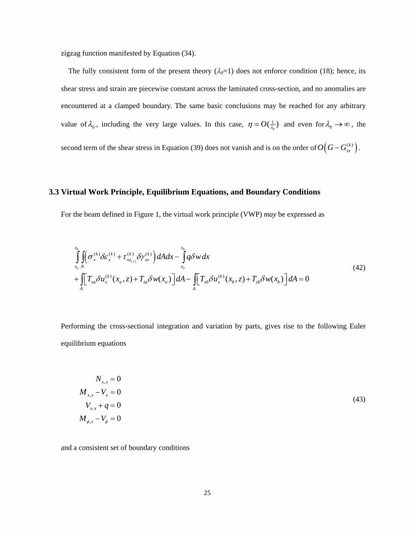
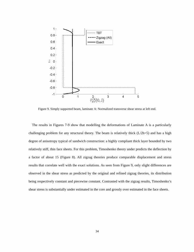
Figure 9. Simply supported beam, laminate A: Normalized transverse shear stress at left end.

The results in Figures 7-9 show that modelling the deformations of Laminate A is a particularly

challenging problem for any structural theory. The beam is relatively thick (L/2h=5) and has a high

degree of anisotropy typical of sandwich construction: a highly compliant thick layer bounded by two

relatively stiff, thin face sheets. For this problem, Timoshenko theory under predicts the deflection by

a factor of about 15 (Figure 8). All zigzag theories produce comparable displacement and stress

results that correlate well with the exact solutions. As seen from Figure 9, only slight differences are

observed in the shear stress as predicted by the original and refined zigzag theories, its distribution

being respectively constant and piecewise constant. Contrasted with the zigzag results, Timoshenko’s

shear stress is substantially under estimated in the core and grossly over estimated in the face sheets.

35

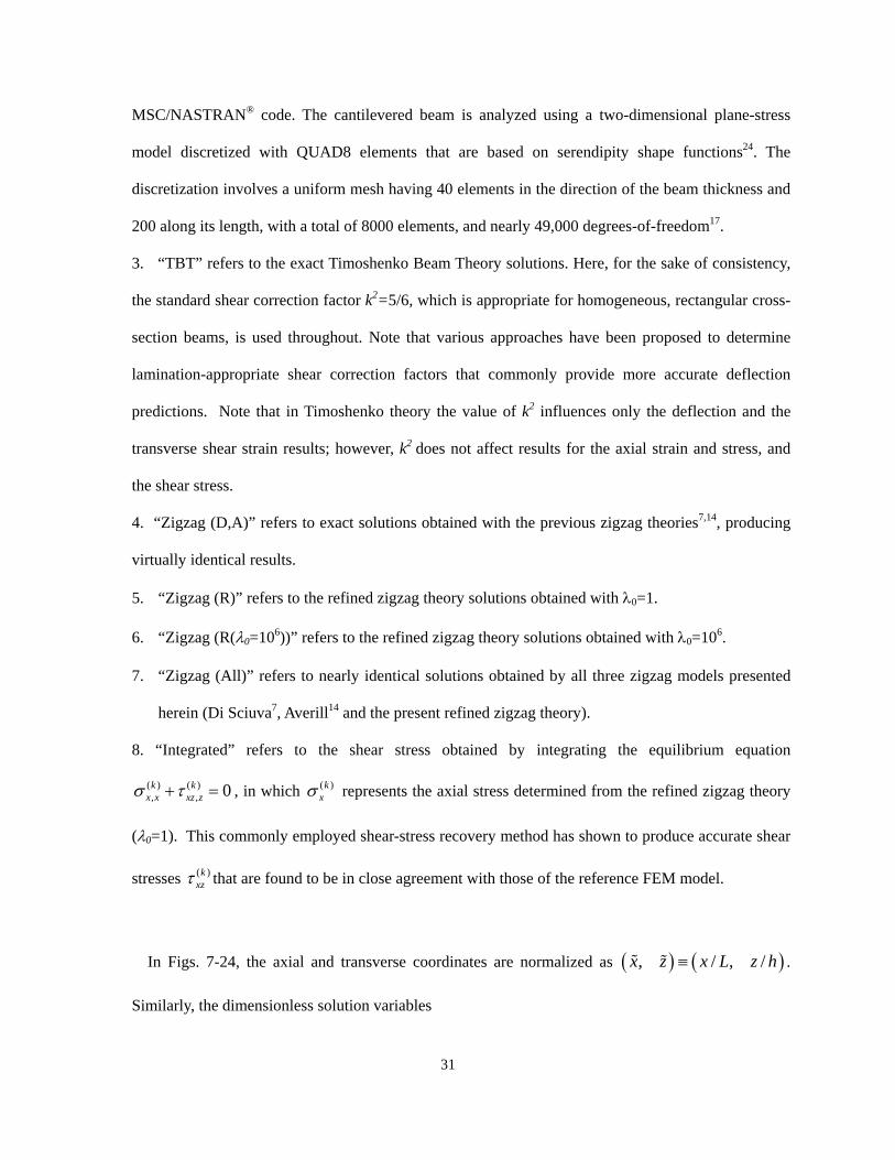
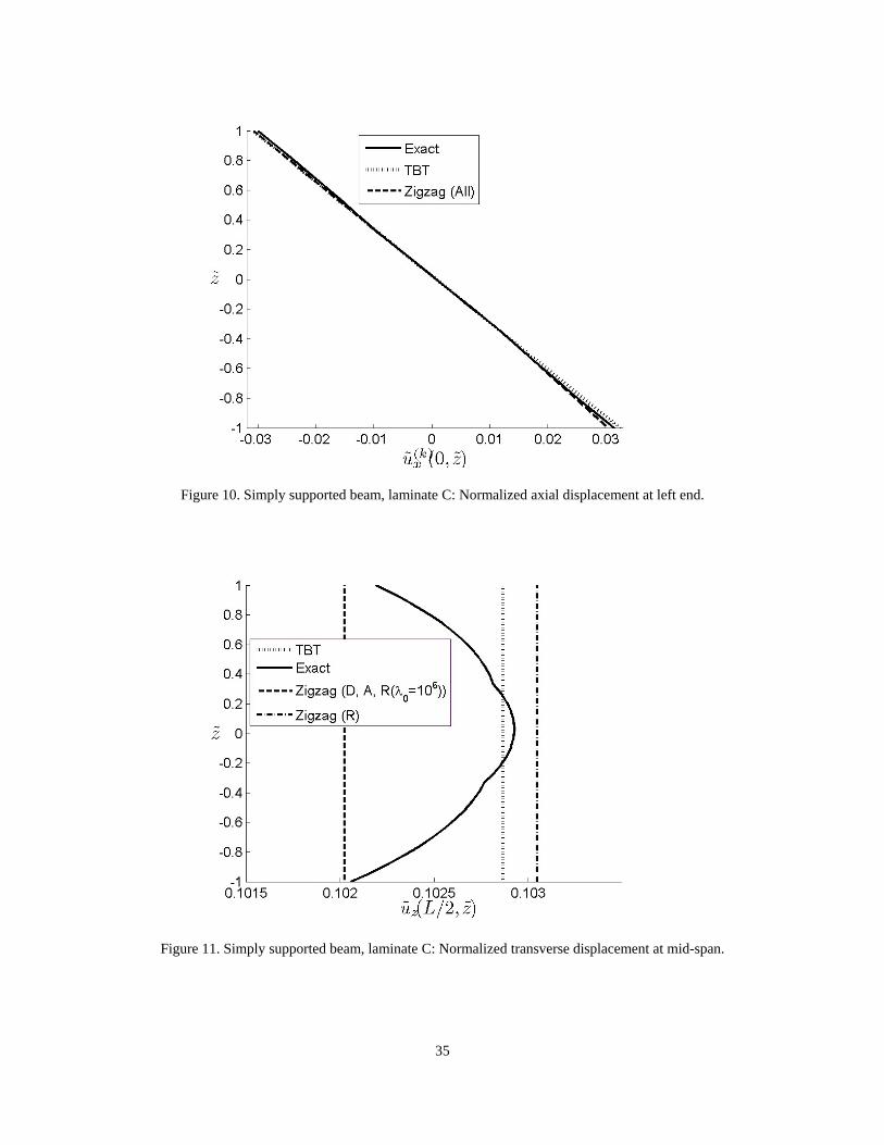
Figure 10. Simply supported beam, laminate C: Normalized axial displacement at left end.

Figure 11. Simply supported beam, laminate C: Normalized transverse displacement at mid-span.

36

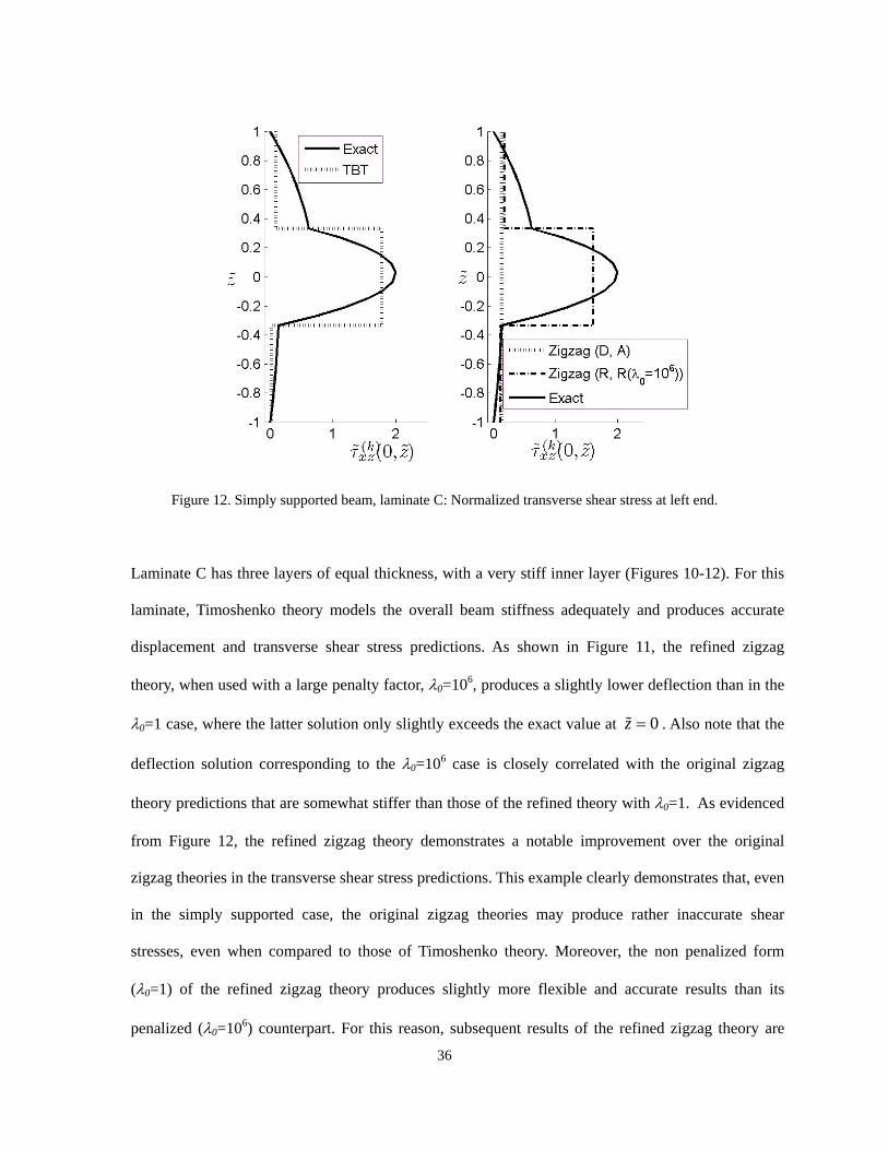
Figure 12. Simply supported beam, laminate C: Normalized transverse shear stress at left end.

Laminate C has three layers of equal thickness, with a very stiff inner layer (Figures 10-12). For this

laminate, Timoshenko theory models the overall beam stiffness adequately and produces accurate

displacement and transverse shear stress predictions. As shown in Figure 11, the refined zigzag

theory, when used with a large penalty factor, λ0=106, produces a slightly lower deflection than in the

λ0=1 case, where the latter solution only slightly exceeds the exact value at 0z = . Also note that the

deflection solution corresponding to the λ0=106 case is closely correlated with the original zigzag

theory predictions that are somewhat stiffer than those of the refined theory with λ0=1. As evidenced

from Figure 12, the refined zigzag theory demonstrates a notable improvement over the original

zigzag theories in the transverse shear stress predictions. This example clearly demonstrates that, even

in the simply supported case, the original zigzag theories may produce rather inaccurate shear

stresses, even when compared to those of Timoshenko theory. Moreover, the non penalized form

(λ0=1) of the refined zigzag theory produces slightly more flexible and accurate results than its

penalized (λ0=106) counterpart. For this reason, subsequent results of the refined zigzag theory are

37

only demonstrated for the non-penalized case (λ0=1).

5.3 Results for Cantilevered Beams

In this section, normalized displacements, stresses, and shear-stress resultants are presented in Figures

13-24 for the clamped beam made of Laminates A and B.

Figure 13. Cantilevered beam, laminate A: Normalized deflection along beam span.

38

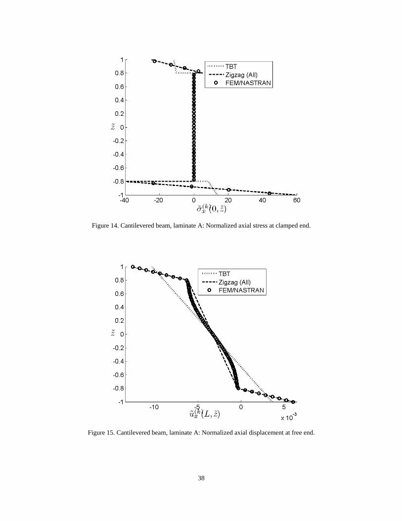
Figure 14. Cantilevered beam, laminate A: Normalized axial stress at clamped end.

Figure 15. Cantilevered beam, laminate A: Normalized axial displacement at free end.

39

Figure 16. Cantilevered beam, laminate A: Normalized axial displacement along top face of beam.

Figure 17. Cantilevered beam, laminate A: Normalized transverse shear stress at clamped end.

40

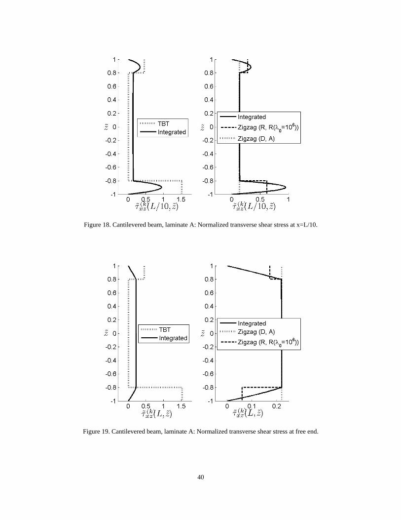
Figure 18. Cantilevered beam, laminate A: Normalized transverse shear stress at x=L/10.

Figure 19. Cantilevered beam, laminate A: Normalized transverse shear stress at free end.

41

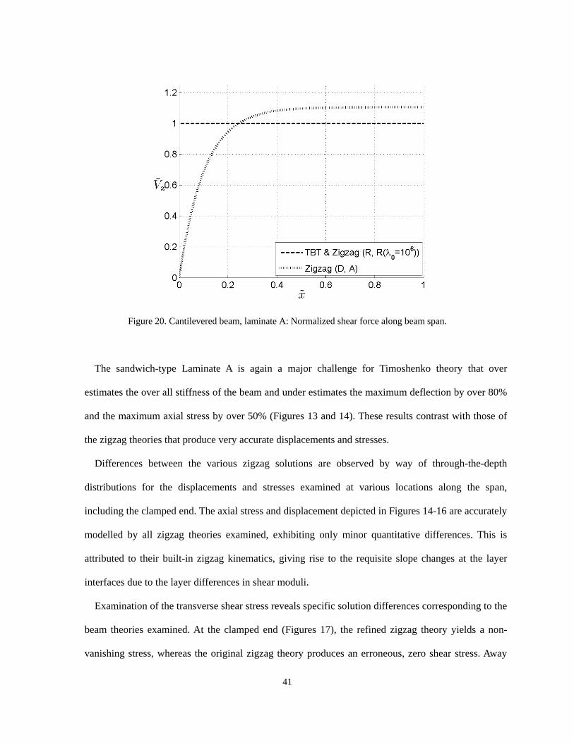
Figure 20. Cantilevered beam, laminate A: Normalized shear force along beam span.

The sandwich-type Laminate A is again a major challenge for Timoshenko theory that over

estimates the over all stiffness of the beam and under estimates the maximum deflection by over 80%

and the maximum axial stress by over 50% (Figures 13 and 14). These results contrast with those of

the zigzag theories that produce very accurate displacements and stresses.

Differences between the various zigzag solutions are observed by way of through-the-depth

distributions for the displacements and stresses examined at various locations along the span,

including the clamped end. The axial stress and displacement depicted in Figures 14-16 are accurately

modelled by all zigzag theories examined, exhibiting only minor quantitative differences. This is

attributed to their built-in zigzag kinematics, giving rise to the requisite slope changes at the layer

interfaces due to the layer differences in shear moduli.

Examination of the transverse shear stress reveals specific solution differences corresponding to the

beam theories examined. At the clamped end (Figures 17), the refined zigzag theory yields a non-

vanishing stress, whereas the original zigzag theory produces an erroneous, zero shear stress. Away

42

from the clamped end (Figures 18 and 19), the shear stress distributions also exhibit substantial

differences. In this problem, the cross-sectional distribution of the shear stress changes significantly

along the beam's span, as expressed by the reference and refined zigzag theory solutions. The original

zigzag theory produces a shear stress that varies in magnitude with respect to the axial coordinate,

while remaining constant across individual cross-sections. The shear stress of the refined zigzag

theory also varies with respect to the axial coordinate; however, it is piecewise constant across the

cross-sections. In contrast, the shear stress due to Timoshenko theory remains constant with respect to

the axial coordinate and exhibits inferior accuracy across the beam’s cross-sections. Finally, the shear

force distribution along the beam’s span clearly pinpoints the transverse shear anomaly inherent

within the original zigzag theory. As shown in Figure 20, the original zigzag theory predicts the

vanishing at the clamped end of the normalized shear force quantity, xV (i.e. the normalized integral

of the shear stress along the beam cross section, see Equation (55) and Equation (21)). Nearly

halfway across the beam, an asymptotic value is achieved that over estimates the correct value by

about 10%. Note, however, that a correct shear force distribution corresponding to Di Sciuva’s theory

is given by the derivative of the bending moment. Both Timoshenko and the refined zigzag theories

give rise to a correct, constant shear force over the entire span of the beam.

43

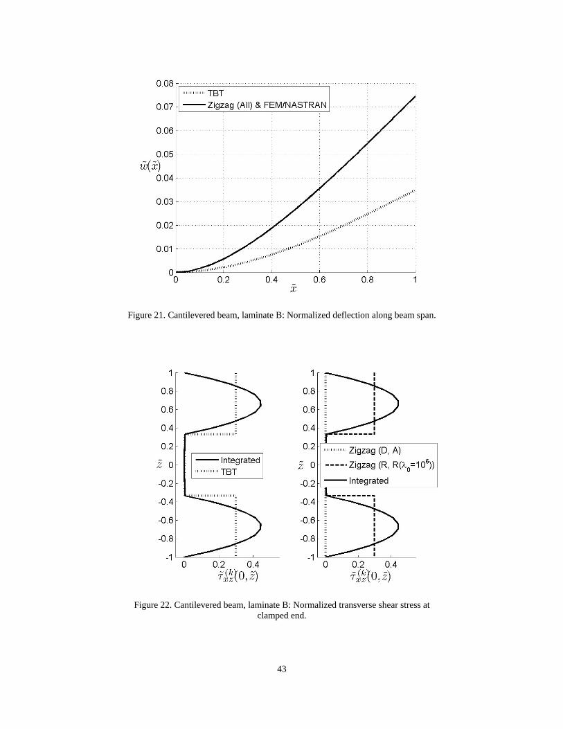
Figure 21. Cantilevered beam, laminate B: Normalized deflection along beam span.

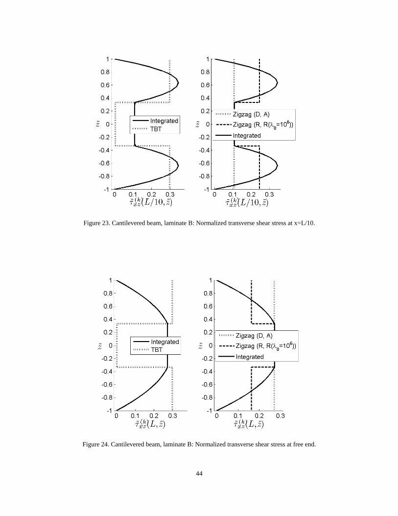
Figure 22. Cantilevered beam, laminate B: Normalized transverse shear stress at clamped end.

44

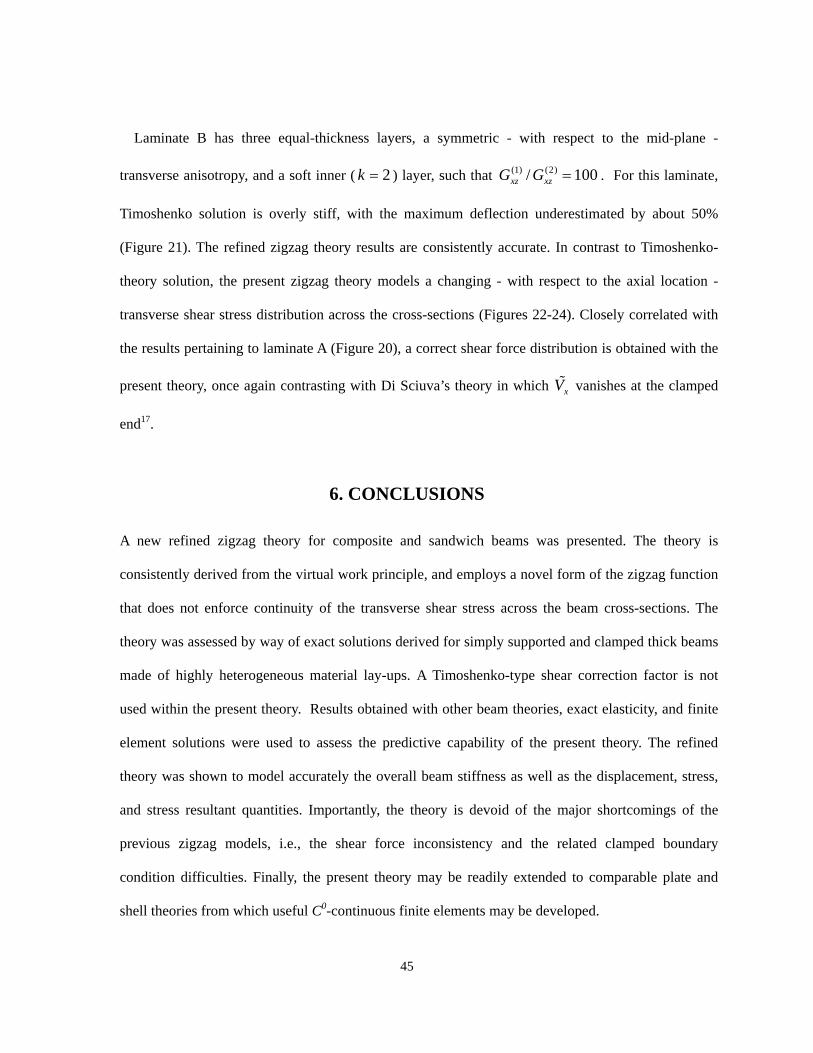
Figure 23. Cantilevered beam, laminate B: Normalized transverse shear stress at x=L/10.

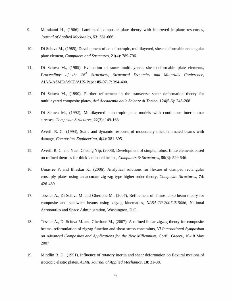
Figure 24. Cantilevered beam, laminate B: Normalized transverse shear stress at free end.

45

Laminate B has three equal-thickness layers, a symmetric - with respect to the mid-plane -

transverse anisotropy, and a soft inner ( 2k = ) layer, such that (1) (2)/ 100xz xzG G = . For this laminate,

Timoshenko solution is overly stiff, with the maximum deflection underestimated by about 50%

(Figure 21). The refined zigzag theory results are consistently accurate. In contrast to Timoshenko-

theory solution, the present zigzag theory models a changing - with respect to the axial location -

transverse shear stress distribution across the cross-sections (Figures 22-24). Closely correlated with

the results pertaining to laminate A (Figure 20), a correct shear force distribution is obtained with the

present theory, once again contrasting with Di Sciuva’s theory in which xV vanishes at the clamped

end17.

6. CONCLUSIONS

A new refined zigzag theory for composite and sandwich beams was presented. The theory is

consistently derived from the virtual work principle, and employs a novel form of the zigzag function

that does not enforce continuity of the transverse shear stress across the beam cross-sections. The

theory was assessed by way of exact solutions derived for simply supported and clamped thick beams

made of highly heterogeneous material lay-ups. A Timoshenko-type shear correction factor is not

used within the present theory. Results obtained with other beam theories, exact elasticity, and finite

element solutions were used to assess the predictive capability of the present theory. The refined

theory was shown to model accurately the overall beam stiffness as well as the displacement, stress,

and stress resultant quantities. Importantly, the theory is devoid of the major shortcomings of the

previous zigzag models, i.e., the shear force inconsistency and the related clamped boundary

condition difficulties. Finally, the present theory may be readily extended to comparable plate and

shell theories from which useful C0-continuous finite elements may be developed.

46

ACKNOWLEDGMENTS

The first author would like to acknowledge the support for this work provided by the Floyd L.

Thompson NASA Fellowship. The third author gratefully acknowledges NIA – National Institute of

Aerospace (Hampton, VA) for inviting and hosting him as a Visiting Researcher in the framework of

“2007 Visitor Program” and acknowledges Politecnico di Torino for supporting his research activity

at NIA in the framework of “Young Researchers Program“ (2006 and 2007).

REFERENCES

1. Timoshenko S., (1921), On the correction for shear of differential equations for transverse

vibrations of prismatic bars, Philos. Mag. Series, 41: 744-746.

2. Liu D. and Li X., (1996), An overall view of laminate theories based on displacement hypothesis,

Journal of Composite Materials, 30(14): 1539-1561.

3. Ambartsumian S. A., (1964), Theory of anisotropic shells, NASA TTF-118.

4. Sun C. T. and Whitney J. M., (1973), Theories for the dynamic response of laminated plates,

AIAA Journal, 11(2): 178-183.

5. Di Sciuva M., (1987), An improved shear-deformation theory for moderately thick multilayered

anisotropic shells and plates, Journal of Applied Mechanics, 54: 589-596.

6. Di Sciuva M., (1984), A refinement of the transverse shear deformation theory for multilayered

orthotropic plates, Proceedings of 7th AIDAA National Congress, October 1983, also published

on L’aerotecnica missili e spazio, 62: 84-92.

7. Di Sciuva M., (1984), A refined transverse shear deformation theory for multilayered anisotropic

plates, Atti Accademia delle Scienze di Torino, 118: 279-295.

8. Di Sciuva M., (1986), Bending, vibration and buckling of simply supported thick multilayered

orthotropic plates: an evaluation of a new displacement model, Journal of Sound and Vibration,

105: 425-442.

47

9. Murakami H., (1986), Laminated composite plate theory with improved in-plane responses,

Journal of Applied Mechanics, 53: 661-666.

10. Di Sciuva M., (1985), Development of an anisotropic, multilayered, shear-deformable rectangular

plate element, Computers and Structures, 21(4): 789-796.

11. Di Sciuva M., (1985), Evaluation of some multilayered, shear-deformable plate elements,

Proceedings of the 26th Structures, Structural Dynamics and Materials Conference,

AIAA/ASME/ASCE/AHS-Paper 85-0717: 394-400.

12. Di Sciuva M., (1990), Further refinement in the transverse shear deformation theory for

multilayered composite plates, Atti Accademia delle Scienze di Torino, 124(5-6): 248-268.

13. Di Sciuva M., (1992), Multilayered anisotropic plate models with continuous interlaminar

stresses, Composite Structures, 22(3): 149-168,

14. Averill R. C., (1994), Static and dynamic response of moderately thick laminated beams with

damage, Composites Engineering, 4(4): 381-395.

15. Averill R. C. and Yuen Cheong Yip, (2006), Development of simple, robust finite elements based

on refined theories for thick laminated beams, Computers & Structures, 59(3): 529-546.

16. Umasree P. and Bhaskar K., (2006), Analytical solutions for flexure of clamped rectangular

cross-ply plates using an accurate zig-zag type higher-order theory, Composite Structures, 74:

426-439.

17. Tessler A., Di Sciuva M. and Gherlone M., (2007), Refinement of Timoshenko beam theory for

composite and sandwich beams using zigzag kinematics, NASA-TP-2007-215086, National

Aeronautics and Space Administration, Washington, D.C.

18. Tessler A., Di Sciuva M. and Gherlone M., (2007), A refined linear zigzag theory for composite

beams: reformulation of zigzag function and shear stress constraints, VI International Symposium

on Advanced Composites and Applications for the New Millennium, Corfù, Greece, 16-18 May

2007

19. Mindlin R. D., (1951), Influence of rotatory inertia and shear deformation on flexural motions of

isotropic elastic plates, ASME Journal of Applied Mechanics, 18: 31-38.

48

20. Reissner E., (1945), The effect of transverse shear deformation on the bending of elastic plates,

ASME Journal of Applied Mechanics, 12: 69-77.

21. Pagano N. J., (1969), Exact solutions for composite laminates in cylindrical bending, Journal of

Composite Materials, 3: 398-411.

22. Di Sciuva M., Gherlone M. and Librescu L., (2002), Implications of damaged interfaces and of

other non-classical effects on the load carrying capacity of multilayered composite shallow shells,

International Journal of Non-Linear Mechanics, 37, 851-867.

23. Zienkiewicz O. C. and Taylor, R. L., (1989), The finite element method, Fourth Edition,

McGraw-Hill Book Company, London

24. MSC/MD-NASTRAN, Reference Guide, Version 2006.0, MSC Software Corporation, Santa

Ana, CA.

49

Table 1. Mechanical material properties.

Material

type

Ex(k ) [GPa]

(Young’s

modulus)

Gxz(k ) [GPa]

(Shear

modulus)

a 73.0 29.2

b 21.9 8.76

c 3.65 1.46

d 0.73 0.292

e 0.219 0.088

f 0.073 0.029

Table 2. Stacking sequences of three-layered laminates

(layer sequence is in the positive z direction).

Laminate Thicknesses [cm] Materials

A (0.20/1.60/0.20) (a/f/b)

B (0.66/0.66/0.66) (b/e/b)

C (0.66/0.66/0.66) (d/a/c)